Assignment 5:

Space-Time Prediction of Bike Share Demand: 2024 Q3 Philadelphia Indego

Author

Sujan Kakumanu

Published

November 17, 2025

Setup

Code
# Core tidyverse
library(tidyverse)
library(lubridate)

# Spatial data
library(sf)
library(tigris)

# Census data
library(tidycensus)

# Weather data
library(riem)  # For Philadelphia weather from ASOS stations

# Visualization
library(viridis)
library(gridExtra)
library(knitr)
library(kableExtra)

# here!
library(here)
# Get rid of scientific notation. We gotta look good!
options(scipen = 999)
Code
plotTheme <- theme(
  plot.title = element_text(size = 14, face = "bold"),
  plot.subtitle = element_text(size = 10),
  plot.caption = element_text(size = 8),
  axis.text.x = element_text(size = 10, angle = 45, hjust = 1),
  axis.text.y = element_text(size = 10),
  axis.title = element_text(size = 11, face = "bold"),
  panel.background = element_blank(),
  panel.grid.major = element_line(colour = "#D0D0D0", size = 0.2),
  panel.grid.minor = element_blank(),
  axis.ticks = element_blank(),
  legend.position = "right"
)

mapTheme <- theme(
  plot.title = element_text(size = 14, face = "bold"),
  plot.subtitle = element_text(size = 10),
  plot.caption = element_text(size = 8),
  axis.line = element_blank(),
  axis.text = element_blank(),
  axis.ticks = element_blank(),
  axis.title = element_blank(),
  panel.background = element_blank(),
  panel.border = element_blank(),
  panel.grid.major = element_line(colour = 'transparent'),
  panel.grid.minor = element_blank(),
  legend.position = "right",
  plot.margin = margin(1, 1, 1, 1, 'cm'),
  legend.key.height = unit(1, "cm"),
  legend.key.width = unit(0.2, "cm")
)

palette5 <- c("#eff3ff", "#bdd7e7", "#6baed6", "#3182bd", "#08519c")
Code
census_api_key(Sys.getenv("MY_CENSUS_API_KEY"), overwrite = TRUE, install = TRUE)

Part 1: Adapting Course Code for Q3 2024 Indego Data

Download data (Q3 2024)

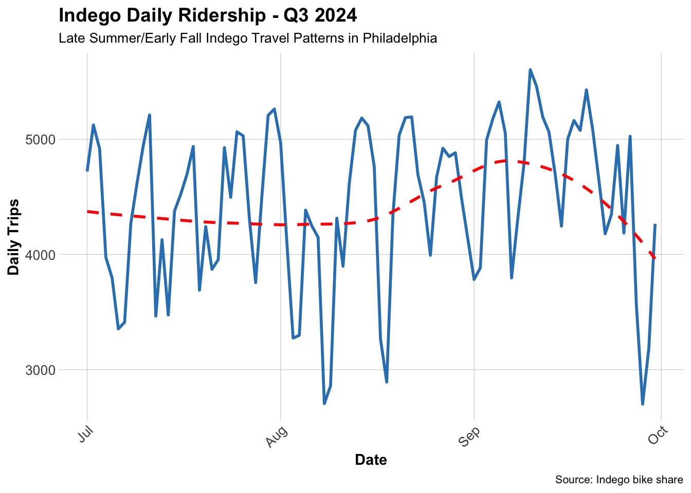
I chose to use Q3 2024 Indego data for this analysis because this period represents a particularly dynamic time of year. Summer travel peaks, schools reopen, the weather begins to change, and numerous major sporting and cultural events take place. These factors create complex and variable travel patterns, making Q3 data more challenging for the models presented in class and highlighting opportunities to explore additional features for improved prediction.

Code
# Read Q3 2024 data
indego <- read_csv("./data/indego-trips-2024-q3.csv")

# Quick look at the data
glimpse(indego)
Rows: 408,408
Columns: 15
$ trip_id             <dbl> 953311130, 953308580, 953309085, 953334269, 953334…
$ duration            <dbl> 5, 3, 2, 12, 22, 47, 111, 7, 1, 8, 6, 2, 20, 246, …
$ start_time          <chr> "7/1/2024 0:02", "7/1/2024 0:03", "7/1/2024 0:04",…
$ end_time            <chr> "7/1/2024 0:07", "7/1/2024 0:06", "7/1/2024 0:06",…
$ start_station       <dbl> 3271, 3304, 3052, 3323, 3209, 3101, 3338, 3373, 33…
$ start_lat           <dbl> 39.94760, 39.94234, 39.94732, 40.02796, 39.94900, …
$ start_lon           <dbl> -75.22946, -75.15399, -75.15695, -75.22770, -75.21…
$ end_station         <dbl> 3338, 3028, 3007, 3323, 3344, 3296, 3258, 3201, 33…
$ end_lat             <dbl> 39.95098, 39.94061, 39.94517, 40.02796, 39.95961, …
$ end_lon             <dbl> -75.23035, -75.14958, -75.15993, -75.22770, -75.23…
$ bike_id             <chr> "03439", "11905", "26031", "19971", "20921", "2241…
$ plan_duration       <dbl> 30, 30, 30, 1, 30, 1, 30, 30, 30, 30, 30, 30, 30, …
$ trip_route_category <chr> "One Way", "One Way", "One Way", "Round Trip", "On…
$ passholder_type     <chr> "Indego30", "Indego30", "Indego30", "Day Pass", "I…
$ bike_type           <chr> "standard", "standard", "electric", "electric", "e…

Data Manipulation and Visualizations

In this section, we create hourly time bins for the Indego data, get basic Census data, load weather data, and produce visualizations. In addition, we join the various data tables to prepare for model creation.

Code
indego <- indego %>%
  mutate(
    # Parse datetime
    start_datetime = mdy_hm(start_time),
    end_datetime = mdy_hm(end_time),
    
    # Create hourly bins
    interval60 = floor_date(start_datetime, unit = "hour"),
    
    # Extract time features
    week = week(interval60),
    month = month(interval60, label = TRUE),
    dotw = wday(interval60, label = TRUE),
    hour = hour(interval60),
    date = as.Date(interval60),
    
    # Create useful indicators
    weekend = ifelse(dotw %in% c("Sat", "Sun"), 1, 0),
    rush_hour = ifelse(hour %in% c(7, 8, 9, 16, 17, 18), 1, 0)
  )

# Look at temporal features
head(indego %>% dplyr::select(start_datetime, interval60, week, dotw, hour, weekend))
# A tibble: 6 × 6
  start_datetime      interval60           week dotw   hour weekend
  <dttm>              <dttm>              <dbl> <ord> <int>   <dbl>
1 2024-07-01 00:02:00 2024-07-01 00:00:00    27 Mon       0       0
2 2024-07-01 00:03:00 2024-07-01 00:00:00    27 Mon       0       0
3 2024-07-01 00:04:00 2024-07-01 00:00:00    27 Mon       0       0
4 2024-07-01 00:05:00 2024-07-01 00:00:00    27 Mon       0       0
5 2024-07-01 00:06:00 2024-07-01 00:00:00    27 Mon       0       0
6 2024-07-01 00:06:00 2024-07-01 00:00:00    27 Mon       0       0
Code
# Get Philadelphia census tracts
philly_census <- get_acs(
  geography = "tract",
  variables = c(
    "B01003_001",  # Total population
    "B19013_001",  # Median household income
    "B08301_001",  # Total commuters
    "B08301_010",  # Commute by transit
    "B02001_002",  # White alone
    "B25077_001"   # Median home value
  ),
  state = "PA",
  county = "Philadelphia",
  year = 2022,
  geometry = TRUE,
  output = "wide",
  progress_bar = F
) %>%
  rename(
    Total_Pop = B01003_001E,
    Med_Inc = B19013_001E,
    Total_Commuters = B08301_001E,
    Transit_Commuters = B08301_010E,
    White_Pop = B02001_002E,
    Med_Home_Value = B25077_001E
  ) %>%
  mutate(
    Percent_Taking_Transit = (Transit_Commuters / Total_Commuters) * 100,
    Percent_White = (White_Pop / Total_Pop) * 100
  ) %>%
  st_transform(crs = 4326, quiet = TRUE)  # WGS84 for lat/lon matching

# Check the data
glimpse(philly_census)
Rows: 408
Columns: 17
$ GEOID                  <chr> "42101001500", "42101001800", "42101002802", "4…
$ NAME                   <chr> "Census Tract 15; Philadelphia County; Pennsylv…
$ Total_Pop              <dbl> 3251, 3300, 5720, 4029, 4415, 1815, 3374, 2729,…
$ B01003_001M            <dbl> 677, 369, 796, 437, 853, 210, 480, 734, 763, 11…
$ Med_Inc                <dbl> 110859, 114063, 78871, 61583, 32347, 48581, 597…
$ B19013_001M            <dbl> 24975, 30714, 20396, 22293, 4840, 13812, 6278, …
$ Total_Commuters        <dbl> 2073, 2255, 3032, 2326, 1980, 969, 2427, 708, 2…
$ B08301_001M            <dbl> 387, 308, 478, 383, 456, 189, 380, 281, 456, 68…
$ Transit_Commuters      <dbl> 429, 123, 685, 506, 534, 192, 658, 218, 438, 51…
$ B08301_010M            <dbl> 188, 66, 219, 144, 285, 71, 278, 184, 176, 235,…
$ White_Pop              <dbl> 2185, 2494, 3691, 3223, 182, 984, 2111, 231, 35…
$ B02001_002M            <dbl> 268, 381, 592, 380, 88, 190, 463, 112, 238, 778…
$ Med_Home_Value         <dbl> 568300, 605000, 350600, 296400, 76600, 289700, …
$ B25077_001M            <dbl> 58894, 34876, 12572, 22333, 10843, 118720, 1506…
$ geometry               <MULTIPOLYGON [°]> MULTIPOLYGON (((-75.16558 3..., MU…
$ Percent_Taking_Transit <dbl> 20.694645, 5.454545, 22.592348, 21.754084, 26.9…
$ Percent_White          <dbl> 67.2100892, 75.5757576, 64.5279720, 79.9950360,…
Code
# Map median income
ggplot() +
  geom_sf(data = philly_census, aes(fill = Med_Inc), color = NA) +
  scale_fill_viridis(
    option = "viridis",
    name = "Median\nIncome",
    labels = scales::dollar
  ) +
  labs(
    title = "Philadelphia Median Household Income by Census Tract",
    subtitle = "Context for understanding bike share demand patterns"
  ) +
  # Stations 
  geom_point(
    data = indego,
    aes(x = start_lon, y = start_lat),
    color = "red", size = 0.25, alpha = 0.6
  ) +
  mapTheme

Code
# Daily trip counts
daily_trips <- indego %>%
  group_by(date) %>%
  summarize(trips = n())

ggplot(daily_trips, aes(x = date, y = trips)) +
  geom_line(color = "#3182bd", linewidth = 1) +
  geom_smooth(se = FALSE, color = "red", linetype = "dashed") +
  labs(
    title = "Indego Daily Ridership - Q3 2024",
    subtitle = "Late Summer/Early Fall Indego Travel Patterns in Philadelphia",
    x = "Date",
    y = "Daily Trips",
    caption = "Source: Indego bike share"
  ) +
  plotTheme

Code
# Get weather from Philadelphia International Airport (KPHL)
# This covers Q3 2024: July 1 - September 30
weather_data <- riem_measures(
  station = "PHL",  # Philadelphia International Airport
  date_start = "2024-07-01",
  date_end = "2024-09-30"
)

# Process weather data
weather_processed <- weather_data %>%
  mutate(
    interval60 = floor_date(valid, unit = "hour"),
    Temperature = tmpf,  # Temperature in Fahrenheit
    Precipitation = ifelse(is.na(p01i), 0, p01i),  # Hourly precip in inches
    Wind_Speed = sknt  # Wind speed in knots
  ) %>%
  dplyr::select(interval60, Temperature, Precipitation, Wind_Speed) %>%
  distinct()

# Check for missing hours and interpolate if needed
weather_complete <- weather_processed %>%
  complete(interval60 = seq(min(interval60), max(interval60), by = "hour")) %>%
  fill(Temperature, Precipitation, Wind_Speed, .direction = "down")

# Look at the weather
summary(weather_complete %>% dplyr::select(Temperature, Precipitation, Wind_Speed))
  Temperature    Precipitation        Wind_Speed    
 Min.   :55.00   Min.   :0.000000   Min.   : 0.000  
 1st Qu.:70.00   1st Qu.:0.000000   1st Qu.: 4.000  
 Median :76.00   Median :0.000000   Median : 7.000  
 Mean   :75.59   Mean   :0.007896   Mean   : 6.893  
 3rd Qu.:81.00   3rd Qu.:0.000000   3rd Qu.: 9.000  
 Max.   :98.00   Max.   :1.250000   Max.   :44.000  
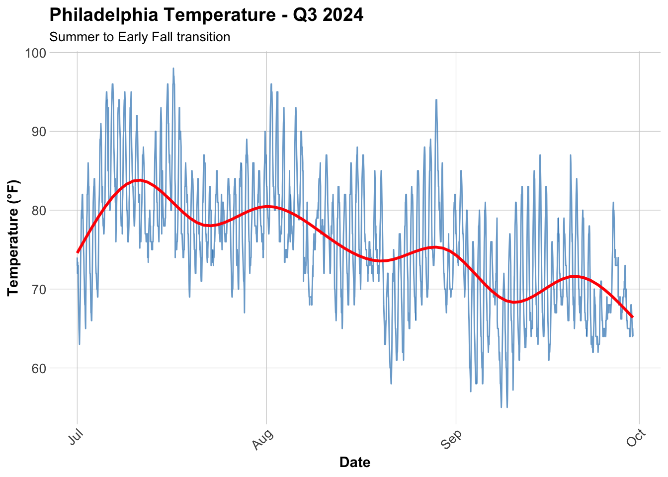
Code
ggplot(weather_complete, aes(x = interval60, y = Temperature)) +
  geom_line(color = "#3182bd", alpha = 0.7) +
  geom_smooth(se = FALSE, color = "red") +
  labs(
    title = "Philadelphia Temperature - Q3 2024",
    subtitle = "Summer to Early Fall transition",
    x = "Date",
    y = "Temperature (°F)"
  ) +
  plotTheme

Code
# Create sf object for stations
stations_sf <- indego %>%
  distinct(start_station, start_lat, start_lon) %>%
  filter(!is.na(start_lat), !is.na(start_lon)) %>%
  st_as_sf(coords = c("start_lon", "start_lat"), crs = 4326)

# Spatial join to get census tract for each station
stations_census <- st_join(stations_sf, philly_census, left = TRUE) %>%
  st_drop_geometry()

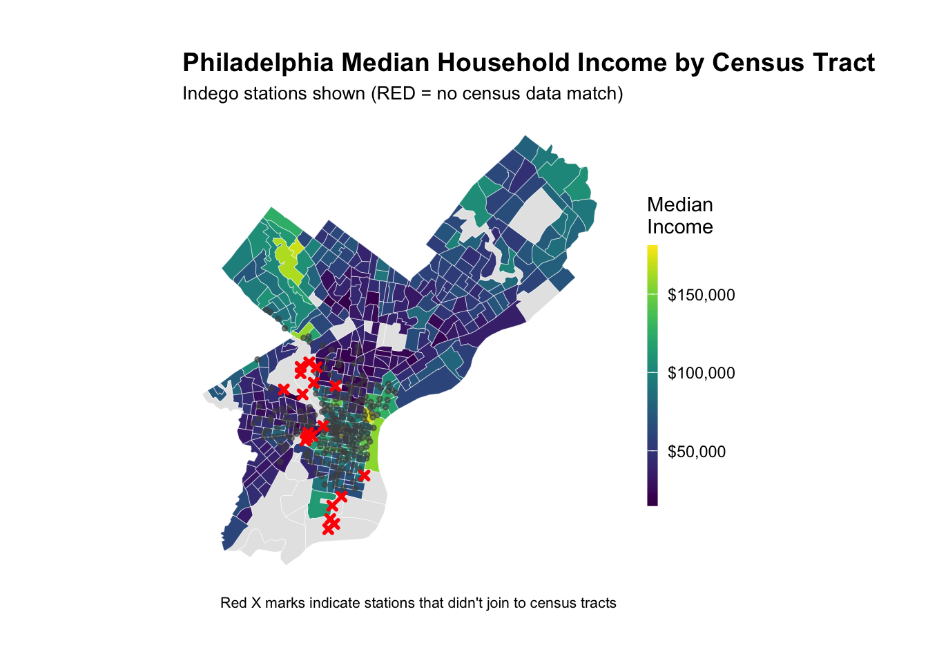
# Look at the result - investigate whether all of the stations joined to census data -- according to the map above there are stations in non-residential tracts.

stations_for_map <- indego %>%
  distinct(start_station, start_lat, start_lon) %>%
  filter(!is.na(start_lat), !is.na(start_lon)) %>%
  left_join(
    stations_census %>% dplyr::select(start_station, Med_Inc),
    by = "start_station"
  ) %>%
  mutate(has_census = !is.na(Med_Inc))

# Add back to trip data
indego_census <- indego %>%
  left_join(
    stations_census %>% 
      dplyr::select(start_station, Med_Inc, Percent_Taking_Transit, 
             Percent_White, Total_Pop),
    by = "start_station"
  )


# Prepare data for visualization
stations_for_map <- indego %>%
  distinct(start_station, start_lat, start_lon) %>%
  filter(!is.na(start_lat), !is.na(start_lon)) %>%
  left_join(
    stations_census %>% dplyr::select(start_station, Med_Inc),
    by = "start_station"
  ) %>%
  mutate(has_census = !is.na(Med_Inc))

# Create the map showing problem stations
ggplot() +
  geom_sf(data = philly_census, aes(fill = Med_Inc), color = "white", size = 0.1) +
  scale_fill_viridis(
    option = "viridis",
    name = "Median\nIncome",
    labels = scales::dollar,
    na.value = "grey90"
  ) +
  # Stations with census data (small grey dots)
  geom_point(
    data = stations_for_map %>% filter(has_census),
    aes(x = start_lon, y = start_lat),
    color = "grey30", size = 1, alpha = 0.6
  ) +
  # Stations WITHOUT census data (red X marks the spot)
  geom_point(
    data = stations_for_map %>% filter(!has_census),
    aes(x = start_lon, y = start_lat),
    color = "red", size = 1, shape = 4, stroke = 1.5
  ) +
  labs(
    title = "Philadelphia Median Household Income by Census Tract",
    subtitle = "Indego stations shown (RED = no census data match)",
    caption = "Red X marks indicate stations that didn't join to census tracts"
  ) +
  mapTheme

Code
# Identify which stations to keep
valid_stations <- stations_census %>%
  filter(!is.na(Med_Inc)) %>%
  pull(start_station)

# Filter trip data to valid stations only
indego_census <- indego %>%
  filter(start_station %in% valid_stations) %>%
  left_join(
    stations_census %>% 
      dplyr::select(start_station, Med_Inc, Percent_Taking_Transit, 
             Percent_White, Total_Pop),
    by = "start_station"
  )
Code
# Aggregating trips to station-hour level
# Count trips by station-hour
trips_panel <- indego_census %>%
  group_by(interval60, start_station, start_lat, start_lon,
           Med_Inc, Percent_Taking_Transit, Percent_White, Total_Pop) %>%
  summarize(Trip_Count = n()) %>%
  ungroup()

# How many station-hour observations?
nrow(trips_panel)
[1] 193072
Code
# How many unique stations?
length(unique(trips_panel$start_station))
[1] 241
Code
# How many unique hours?
length(unique(trips_panel$interval60))
[1] 2202
Code
# Calculate expected panel size
n_stations <- length(unique(trips_panel$start_station))
n_hours <- length(unique(trips_panel$interval60))
expected_rows <- n_stations * n_hours

cat("Expected panel rows:", format(expected_rows, big.mark = ","), "\n")
Expected panel rows: 530,682 
Code
cat("Current rows:", format(nrow(trips_panel), big.mark = ","), "\n")
Current rows: 193,072 
Code
cat("Missing rows:", format(expected_rows - nrow(trips_panel), big.mark = ","), "\n")
Missing rows: 337,610 
Code
# Create complete panel
study_panel <- expand.grid(
  interval60 = unique(trips_panel$interval60),
  start_station = unique(trips_panel$start_station)
) %>%
  # Join trip counts
  left_join(trips_panel, by = c("interval60", "start_station")) %>%
  # Replace NA trip counts with 0
  mutate(Trip_Count = replace_na(Trip_Count, 0))

# Fill in station attributes (they're the same for all hours)
station_attributes <- trips_panel %>%
  group_by(start_station) %>%
  summarize(
    start_lat = first(start_lat),
    start_lon = first(start_lon),
    Med_Inc = first(Med_Inc),
    Percent_Taking_Transit = first(Percent_Taking_Transit),
    Percent_White = first(Percent_White),
    Total_Pop = first(Total_Pop)
  )

study_panel <- study_panel %>%
  left_join(station_attributes, by = "start_station")

# Verify we have complete panel
cat("Complete panel rows:", format(nrow(study_panel), big.mark = ","), "\n")
Complete panel rows: 530,682 
Code
study_panel <- study_panel %>%
  mutate(
    week = week(interval60),
    month = month(interval60, label = TRUE),
    dotw = wday(interval60, label = TRUE),
    hour = hour(interval60),
    date = as.Date(interval60),
    weekend = ifelse(dotw %in% c("Sat", "Sun"), 1, 0),
    rush_hour = ifelse(hour %in% c(7, 8, 9, 16, 17, 18), 1, 0)
  )
Code
study_panel <- study_panel %>%
  left_join(weather_complete, by = "interval60")

# Check for missing values
summary(study_panel %>% dplyr::select(Trip_Count, Temperature, Precipitation))
   Trip_Count       Temperature    Precipitation   
 Min.   : 0.0000   Min.   :55.00   Min.   :0.0000  
 1st Qu.: 0.0000   1st Qu.:70.00   1st Qu.:0.0000  
 Median : 0.0000   Median :76.00   Median :0.0000  
 Mean   : 0.7068   Mean   :75.59   Mean   :0.0079  
 3rd Qu.: 1.0000   3rd Qu.:81.00   3rd Qu.:0.0000  
 Max.   :24.0000   Max.   :98.00   Max.   :1.2500  
                   NA's   :5784    NA's   :5784    
Code
# Sort by station and time
study_panel <- study_panel %>%
  arrange(start_station, interval60)

# Create lag variables WITHIN each station
study_panel <- study_panel %>%
  group_by(start_station) %>%
  mutate(
    lag1Hour = lag(Trip_Count, 1),
    lag2Hours = lag(Trip_Count, 2),
    lag3Hours = lag(Trip_Count, 3),
    lag12Hours = lag(Trip_Count, 12),
    lag1day = lag(Trip_Count, 24)
  ) %>%
  ungroup()

# Remove rows with NA lags (first 24 hours for each station)
study_panel_complete <- study_panel %>%
  filter(!is.na(lag1day))

cat("Rows after removing NA lags:", format(nrow(study_panel_complete), big.mark = ","), "\n")
Rows after removing NA lags: 646,362 
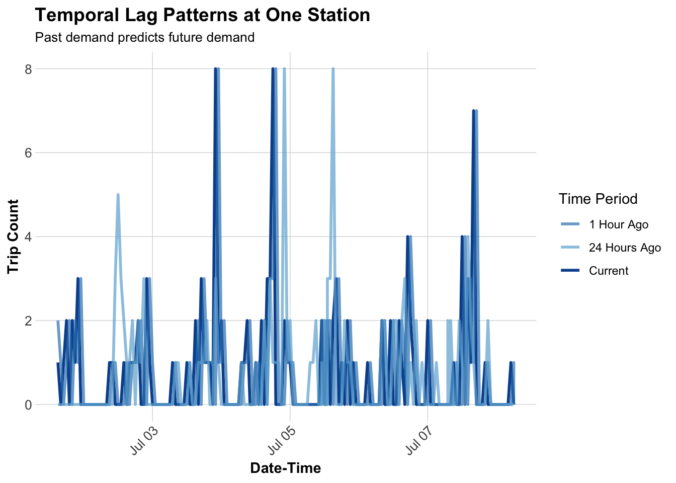
Code
# Sample one station to visualize
example_station <- study_panel_complete %>%
  filter(start_station == first(start_station)) %>%
  head(168)  # One week

# Plot actual vs lagged demand
ggplot(example_station, aes(x = interval60)) +
  geom_line(aes(y = Trip_Count, color = "Current"), linewidth = 1) +
  geom_line(aes(y = lag1Hour, color = "1 Hour Ago"), linewidth = 1, alpha = 0.7) +
  geom_line(aes(y = lag1day, color = "24 Hours Ago"), linewidth = 1, alpha = 0.7) +
  scale_color_manual(values = c(
    "Current" = "#08519c",
    "1 Hour Ago" = "#3182bd",
    "24 Hours Ago" = "#6baed6"
  )) +
  labs(
    title = "Temporal Lag Patterns at One Station",
    subtitle = "Past demand predicts future demand",
    x = "Date-Time",
    y = "Trip Count",
    color = "Time Period"
  ) +
  plotTheme

Code
# Split by week
# Q3 2024 has weeks ~27–39 (July–September)
# Train on weeks 27–35 (July → late August)
# Test on weeks 36–39 (September)

# Which stations have trips in BOTH early and late periods?
early_stations <- study_panel_complete %>%
  filter(week < 36) %>%        # weeks 27–35
  filter(Trip_Count > 0) %>%
  distinct(start_station) %>%
  pull(start_station)

late_stations <- study_panel_complete %>%
  filter(week >= 36) %>%       # weeks 36–39
  filter(Trip_Count > 0) %>%
  distinct(start_station) %>%
  pull(start_station)

# Keep only stations that appear in BOTH periods
common_stations <- intersect(early_stations, late_stations)

# Filter panel to only common stations
study_panel_complete <- study_panel_complete %>%
  filter(start_station %in% common_stations)

# NOW create train/test split
train <- study_panel_complete %>%
  filter(week < 36)

test <- study_panel_complete %>%
  filter(week >= 36)

cat("Training observations:", format(nrow(train), big.mark = ","), "\n")
Training observations: 426,995 
Code
cat("Testing observations:", format(nrow(test), big.mark = ","), "\n")
Testing observations: 203,275 
Code
cat("Training date range:", min(train$date), "to", max(train$date), "\n")
Training date range: 19905 to 19967 
Code
cat("Testing date range:", min(test$date), "to", max(test$date), "\n")
Testing date range: 19968 to 19996 

Build Predictive Models

We’ll build 5 models with increasing complexity to see what improves predictions.

Model 1: Baseline (Time + Weather)

Code
# Create day of week factor with treatment (dummy) coding
train <- train %>%
  mutate(dotw_simple = factor(dotw, levels = c("Mon", "Tue", "Wed", "Thu", "Fri", "Sat", "Sun")))

# Set contrasts to treatment coding (dummy variables)
contrasts(train$dotw_simple) <- contr.treatment(7)

# Now run the model
model1 <- lm(
  Trip_Count ~ as.factor(hour) + dotw_simple + Temperature + Precipitation,
  data = train
)

summary(model1)

Call:
lm(formula = Trip_Count ~ as.factor(hour) + dotw_simple + Temperature + 
    Precipitation, data = train)

Residuals:
    Min      1Q  Median      3Q     Max 
-1.6699 -0.7865 -0.1952  0.1894 23.4789 

Coefficients:
                    Estimate Std. Error t value             Pr(>|t|)    
(Intercept)        0.1907758  0.0300331   6.352  0.00000000021248305 ***
as.factor(hour)1  -0.0983522  0.0126388  -7.782  0.00000000000000717 ***
as.factor(hour)2  -0.1241393  0.0128704  -9.645 < 0.0000000000000002 ***
as.factor(hour)3  -0.1764085  0.0132525 -13.311 < 0.0000000000000002 ***
as.factor(hour)4  -0.1584485  0.0130394 -12.152 < 0.0000000000000002 ***
as.factor(hour)5  -0.0294027  0.0128895  -2.281              0.02254 *  
as.factor(hour)6   0.2317631  0.0130472  17.763 < 0.0000000000000002 ***
as.factor(hour)7   0.5137459  0.0130438  39.386 < 0.0000000000000002 ***
as.factor(hour)8   0.9225191  0.0130186  70.862 < 0.0000000000000002 ***
as.factor(hour)9   0.6732479  0.0131111  51.349 < 0.0000000000000002 ***
as.factor(hour)10  0.5471686  0.0129073  42.392 < 0.0000000000000002 ***
as.factor(hour)11  0.5675162  0.0130596  43.456 < 0.0000000000000002 ***
as.factor(hour)12  0.6846655  0.0129836  52.733 < 0.0000000000000002 ***
as.factor(hour)13  0.6714138  0.0127505  52.658 < 0.0000000000000002 ***
as.factor(hour)14  0.7408376  0.0127923  57.913 < 0.0000000000000002 ***
as.factor(hour)15  0.7774720  0.0127123  61.159 < 0.0000000000000002 ***
as.factor(hour)16  0.9943089  0.0130734  76.056 < 0.0000000000000002 ***
as.factor(hour)17  1.3409901  0.0131651 101.859 < 0.0000000000000002 ***
as.factor(hour)18  1.0705918  0.0132411  80.854 < 0.0000000000000002 ***
as.factor(hour)19  0.8329199  0.0130579  63.787 < 0.0000000000000002 ***
as.factor(hour)20  0.6032729  0.0126386  47.733 < 0.0000000000000002 ***
as.factor(hour)21  0.3788668  0.0127578  29.697 < 0.0000000000000002 ***
as.factor(hour)22  0.2653238  0.0124655  21.285 < 0.0000000000000002 ***
as.factor(hour)23  0.1487921  0.0132089  11.264 < 0.0000000000000002 ***
dotw_simple2       0.0666909  0.0073090   9.125 < 0.0000000000000002 ***
dotw_simple3       0.0674092  0.0071645   9.409 < 0.0000000000000002 ***
dotw_simple4      -0.0019771  0.0071948  -0.275              0.78348    
dotw_simple5      -0.0558390  0.0071752  -7.782  0.00000000000000714 ***
dotw_simple6      -0.0528449  0.0072359  -7.303  0.00000000000028159 ***
dotw_simple7      -0.1200020  0.0071570 -16.767 < 0.0000000000000002 ***
Temperature        0.0007438  0.0003513   2.118              0.03421 *  
Precipitation     -0.0900337  0.0322306  -2.793              0.00522 ** 
---
Signif. codes:  0 '***' 0.001 '**' 0.01 '*' 0.05 '.' 0.1 ' ' 1

Residual standard error: 1.208 on 426963 degrees of freedom
Multiple R-squared:  0.1081,    Adjusted R-squared:  0.1081 
F-statistic:  1670 on 31 and 426963 DF,  p-value: < 0.00000000000000022

Model 2: Add Temporal Lags

Code
model2 <- lm(
  Trip_Count ~ as.factor(hour) + dotw_simple + Temperature + Precipitation +
    lag1Hour + lag3Hours + lag1day,
  data = train
)

summary(model2)

Call:
lm(formula = Trip_Count ~ as.factor(hour) + dotw_simple + Temperature + 
    Precipitation + lag1Hour + lag3Hours + lag1day, data = train)

Residuals:
    Min      1Q  Median      3Q     Max 
-7.8107 -0.4918 -0.1362  0.1938 20.2697 

Coefficients:
                    Estimate Std. Error t value             Pr(>|t|)    
(Intercept)        0.0786561  0.0260209   3.023             0.002505 ** 
as.factor(hour)1  -0.0305732  0.0109513  -2.792             0.005243 ** 
as.factor(hour)2  -0.0204266  0.0111573  -1.831             0.067134 .  
as.factor(hour)3  -0.0442404  0.0114929  -3.849             0.000118 ***
as.factor(hour)4  -0.0252562  0.0113182  -2.231             0.025650 *  
as.factor(hour)5   0.0929684  0.0111892   8.309 < 0.0000000000000002 ***
as.factor(hour)6   0.2902340  0.0113286  25.620 < 0.0000000000000002 ***
as.factor(hour)7   0.4463363  0.0113331  39.384 < 0.0000000000000002 ***
as.factor(hour)8   0.6894525  0.0113249  60.879 < 0.0000000000000002 ***
as.factor(hour)9   0.3025745  0.0114123  26.513 < 0.0000000000000002 ***
as.factor(hour)10  0.2552202  0.0112091  22.769 < 0.0000000000000002 ***
as.factor(hour)11  0.2808766  0.0113442  24.759 < 0.0000000000000002 ***
as.factor(hour)12  0.4037984  0.0112751  35.813 < 0.0000000000000002 ***
as.factor(hour)13  0.3690166  0.0110804  33.303 < 0.0000000000000002 ***
as.factor(hour)14  0.4126816  0.0111195  37.113 < 0.0000000000000002 ***
as.factor(hour)15  0.4478829  0.0110488  40.537 < 0.0000000000000002 ***
as.factor(hour)16  0.6138841  0.0113736  53.974 < 0.0000000000000002 ***
as.factor(hour)17  0.8694958  0.0114777  75.755 < 0.0000000000000002 ***
as.factor(hour)18  0.4952317  0.0115800  42.766 < 0.0000000000000002 ***
as.factor(hour)19  0.3802954  0.0113812  33.414 < 0.0000000000000002 ***
as.factor(hour)20  0.2327581  0.0110158  21.129 < 0.0000000000000002 ***
as.factor(hour)21  0.1360156  0.0110822  12.273 < 0.0000000000000002 ***
as.factor(hour)22  0.1435774  0.0108077  13.285 < 0.0000000000000002 ***
as.factor(hour)23  0.0581483  0.0114470   5.080        0.00000037806 ***
dotw_simple2       0.0211603  0.0063332   3.341             0.000834 ***
dotw_simple3       0.0121472  0.0062096   1.956             0.050444 .  
dotw_simple4      -0.0313699  0.0062374  -5.029        0.00000049236 ***
dotw_simple5      -0.0342061  0.0062178  -5.501        0.00000003772 ***
dotw_simple6      -0.0381694  0.0062715  -6.086        0.00000000116 ***
dotw_simple7      -0.0578545  0.0062045  -9.325 < 0.0000000000000002 ***
Temperature       -0.0011927  0.0003044  -3.918        0.00008929826 ***
Precipitation      0.0618332  0.0279337   2.214             0.026859 *  
lag1Hour           0.3767247  0.0014350 262.520 < 0.0000000000000002 ***
lag3Hours          0.1281318  0.0014104  90.845 < 0.0000000000000002 ***
lag1day            0.1448192  0.0013178 109.891 < 0.0000000000000002 ***
---
Signif. codes:  0 '***' 0.001 '**' 0.01 '*' 0.05 '.' 0.1 ' ' 1

Residual standard error: 1.046 on 426960 degrees of freedom
Multiple R-squared:  0.3307,    Adjusted R-squared:  0.3306 
F-statistic:  6204 on 34 and 426960 DF,  p-value: < 0.00000000000000022

Model 3: Add Demographics

Code
model3 <- lm(
  Trip_Count ~ as.factor(hour) + dotw_simple + Temperature + Precipitation +
    lag1Hour + lag3Hours + lag1day +
    Med_Inc.x + Percent_Taking_Transit.y + Percent_White.y,
  data = train
)

summary(model3)

Call:
lm(formula = Trip_Count ~ as.factor(hour) + dotw_simple + Temperature + 
    Precipitation + lag1Hour + lag3Hours + lag1day + Med_Inc.x + 
    Percent_Taking_Transit.y + Percent_White.y, data = train)

Residuals:
    Min      1Q  Median      3Q     Max 
-6.2111 -0.7300 -0.2851  0.4535 20.1808 

Coefficients:
                              Estimate    Std. Error t value
(Intercept)               0.7753069602  0.0569020384  13.625
as.factor(hour)1          0.0336186991  0.0377901050   0.890
as.factor(hour)2          0.0487073183  0.0413330957   1.178
as.factor(hour)3         -0.0447495990  0.0512983936  -0.872
as.factor(hour)4         -0.0853899954  0.0449166805  -1.901
as.factor(hour)5          0.0090602737  0.0336006738   0.270
as.factor(hour)6          0.2842169220  0.0300200985   9.468
as.factor(hour)7          0.4337803415  0.0285613711  15.188
as.factor(hour)8          0.7064995985  0.0276799079  25.524
as.factor(hour)9          0.1844068018  0.0278801834   6.614
as.factor(hour)10         0.1621109760  0.0278934198   5.812
as.factor(hour)11         0.2192858261  0.0280222299   7.825
as.factor(hour)12         0.3325947064  0.0276609321  12.024
as.factor(hour)13         0.2872568947  0.0274476983  10.466
as.factor(hour)14         0.3479704696  0.0273979816  12.701
as.factor(hour)15         0.4017667237  0.0273268893  14.702
as.factor(hour)16         0.5988989541  0.0274585814  21.811
as.factor(hour)17         0.9434659166  0.0273617566  34.481
as.factor(hour)18         0.4673445776  0.0276570683  16.898
as.factor(hour)19         0.3343084390  0.0277357348  12.053
as.factor(hour)20         0.1706327318  0.0277943019   6.139
as.factor(hour)21         0.1102048135  0.0286974725   3.840
as.factor(hour)22         0.1561084025  0.0289810638   5.387
as.factor(hour)23         0.0782781732  0.0312446790   2.505
dotw_simple2              0.0344509932  0.0126053537   2.733
dotw_simple3              0.0322340427  0.0124474335   2.590
dotw_simple4             -0.0390989926  0.0125576132  -3.114
dotw_simple5             -0.0780794855  0.0125351420  -6.229
dotw_simple6             -0.0194068626  0.0129583220  -1.498
dotw_simple7             -0.0516221889  0.0128483055  -4.018
Temperature               0.0008575906  0.0006077802   1.411
Precipitation            -0.3729418315  0.0699319873  -5.333
lag1Hour                  0.2752540882  0.0021977530 125.243
lag3Hours                 0.0856650838  0.0022698183  37.741
lag1day                   0.1119405714  0.0021580117  51.872
Med_Inc.x                 0.0000007633  0.0000001152   6.623
Percent_Taking_Transit.y -0.0038729434  0.0004225528  -9.166
Percent_White.y           0.0029655331  0.0002117857  14.003
                                     Pr(>|t|)    
(Intercept)              < 0.0000000000000002 ***
as.factor(hour)1                     0.373673    
as.factor(hour)2                     0.238635    
as.factor(hour)3                     0.383025    
as.factor(hour)4                     0.057294 .  
as.factor(hour)5                     0.787433    
as.factor(hour)6         < 0.0000000000000002 ***
as.factor(hour)7         < 0.0000000000000002 ***
as.factor(hour)8         < 0.0000000000000002 ***
as.factor(hour)9          0.00000000003746268 ***
as.factor(hour)10         0.00000000619258551 ***
as.factor(hour)11         0.00000000000000509 ***
as.factor(hour)12        < 0.0000000000000002 ***
as.factor(hour)13        < 0.0000000000000002 ***
as.factor(hour)14        < 0.0000000000000002 ***
as.factor(hour)15        < 0.0000000000000002 ***
as.factor(hour)16        < 0.0000000000000002 ***
as.factor(hour)17        < 0.0000000000000002 ***
as.factor(hour)18        < 0.0000000000000002 ***
as.factor(hour)19        < 0.0000000000000002 ***
as.factor(hour)20         0.00000000083178003 ***
as.factor(hour)21                    0.000123 ***
as.factor(hour)22         0.00000007192152554 ***
as.factor(hour)23                    0.012235 *  
dotw_simple2                         0.006276 ** 
dotw_simple3                         0.009609 ** 
dotw_simple4                         0.001849 ** 
dotw_simple5              0.00000000047108679 ***
dotw_simple6                         0.134230    
dotw_simple7              0.00005876669231491 ***
Temperature                          0.158240    
Precipitation             0.00000009678053825 ***
lag1Hour                 < 0.0000000000000002 ***
lag3Hours                < 0.0000000000000002 ***
lag1day                  < 0.0000000000000002 ***
Med_Inc.x                 0.00000000003529142 ***
Percent_Taking_Transit.y < 0.0000000000000002 ***
Percent_White.y          < 0.0000000000000002 ***
---
Signif. codes:  0 '***' 0.001 '**' 0.01 '*' 0.05 '.' 0.1 ' ' 1

Residual standard error: 1.28 on 154100 degrees of freedom
  (272857 observations deleted due to missingness)
Multiple R-squared:  0.2188,    Adjusted R-squared:  0.2186 
F-statistic:  1167 on 37 and 154100 DF,  p-value: < 0.00000000000000022

Model 4: Add Station Fixed Effects

Code
model4 <- lm(
  Trip_Count ~ as.factor(hour) + dotw_simple + Temperature + Precipitation +
    lag1Hour + lag3Hours + lag1day +
    Med_Inc.x + Percent_Taking_Transit.y + Percent_White.y +
    as.factor(start_station),
  data = train
)

# Summary too long with all station dummies, just show key metrics
cat("Model 4 R-squared:", summary(model4)$r.squared, "\n")
Model 4 R-squared: 0.2481647 
Code
cat("Model 4 Adj R-squared:", summary(model4)$adj.r.squared, "\n")
Model 4 Adj R-squared: 0.2468552 

Model 5: Add Rush Hour Interaction

Code
model5 <- lm(
  Trip_Count ~ as.factor(hour) + dotw_simple + Temperature + Precipitation +
    lag1Hour + lag3Hours + lag1day + rush_hour + as.factor(month) +
    Med_Inc.x + Percent_Taking_Transit.y + Percent_White.y +
    as.factor(start_station) +
    rush_hour * weekend,  # Rush hour effects different on weekends
  data = train
)

cat("Model 5 R-squared:", summary(model5)$r.squared, "\n")
Model 5 R-squared: 0.2530642 
Code
cat("Model 5 Adj R-squared:", summary(model5)$adj.r.squared, "\n")
Model 5 Adj R-squared: 0.2517486 

Model Evaluation

Calculate Predictions and MAE

Code
# Get predictions on test set

# Create day of week factor with treatment (dummy) coding
test <- test %>%
  mutate(dotw_simple = factor(dotw, levels = c("Mon", "Tue", "Wed", "Thu", "Fri", "Sat", "Sun")))

# Set contrasts to treatment coding (dummy variables)
contrasts(test$dotw_simple) <- contr.treatment(7)

test <- test %>%
  mutate(
    pred1 = predict(model1, newdata = test),
    pred2 = predict(model2, newdata = test),
    pred3 = predict(model3, newdata = test),
    pred4 = predict(model4, newdata = test),
    pred5 = predict(model5, newdata = test)
  )

# Calculate MAE for each model
mae_results <- data.frame(
  Model = c(
    "1. Time + Weather",
    "2. + Temporal Lags",
    "3. + Demographics",
    "4. + Station FE",
    "5. + Rush Hour Interaction"
  ),
  MAE = c(
    mean(abs(test$Trip_Count - test$pred1), na.rm = TRUE),
    mean(abs(test$Trip_Count - test$pred2), na.rm = TRUE),
    mean(abs(test$Trip_Count - test$pred3), na.rm = TRUE),
    mean(abs(test$Trip_Count - test$pred4), na.rm = TRUE),
    mean(abs(test$Trip_Count - test$pred5), na.rm = TRUE)
  )
)

kable(mae_results, 
      digits = 2,
      caption = "Mean Absolute Error by Model (Test Set)",
      col.names = c("Model", "MAE (trips)")) %>%
  kable_styling(bootstrap_options = c("striped", "hover"))
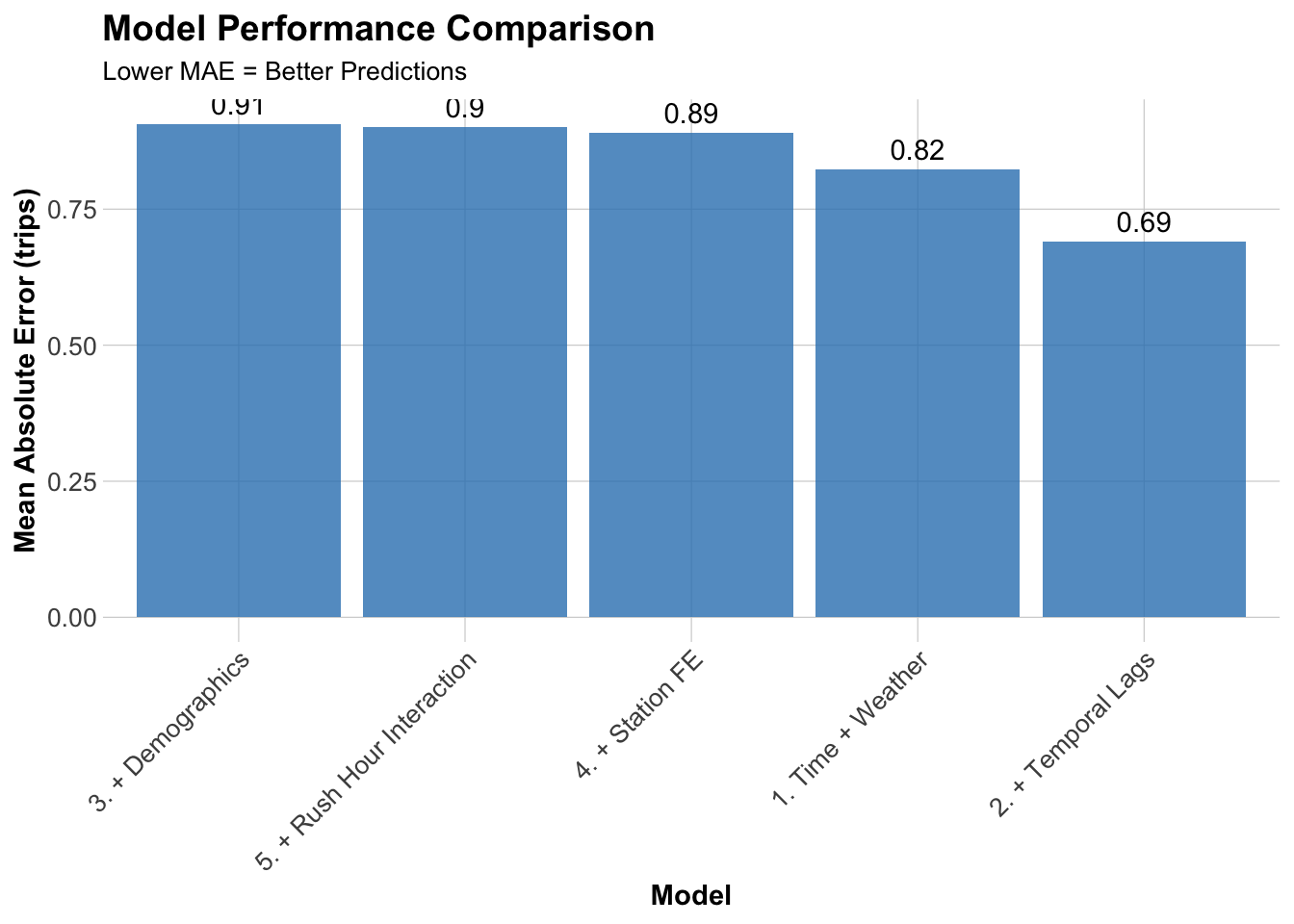
Mean Absolute Error by Model (Test Set)
Model MAE (trips)
1. Time + Weather 0.82
2. + Temporal Lags 0.69
3. + Demographics 0.91
4. + Station FE 0.89
5. + Rush Hour Interaction 0.90

Visualize Model Comparison

Code
ggplot(mae_results, aes(x = reorder(Model, -MAE), y = MAE)) +
  geom_col(fill = "#3182bd", alpha = 0.8) +
  geom_text(aes(label = round(MAE, 2)), vjust = -0.5) +
  labs(
    title = "Model Performance Comparison",
    subtitle = "Lower MAE = Better Predictions",
    x = "Model",
    y = "Mean Absolute Error (trips)"
  ) +
  plotTheme +
  theme(axis.text.x = element_text(angle = 45, hjust = 1))

Compare results to Q1 2025 (found in the course repository):

Model Results Comparison

Model Step Q1 2025 Q3 2024
Time + Weather 0.60 0.82
+ Temporal Lags 0.50 0.69
+ Demographics 0.74 0.91
+ Station FE 0.73 0.89
+ Rush Hour Interaction 0.73 0.90

As seen in the table above, the MAE values for the Q3 2024 models are consistently worse than those of the Q1 2025 models. This suggests that the models are performing worse on the Q3 2024 data, with predicted values further away from actual values. This could be attributed to many reasons. First, Q3 2024 covers a very chaotic period of the calendar year: peak summer travel, the return to school (both K-12 and Higher Education), the start of the fall sports season, etc. This will naturally result in different travel patterns than Q1 2025, which mostly covers the worst of winter weather in the city and also when less events are occurring.

Temporal patterns are different between the two quarters. In both models, performance is improved by including temporal lags which suggests that past ridership consistently helps predict current ridership. At the same time, there is a greater improvement in MAE by adding temporal lags in the Q3 2024 data. This may suggest a higher predictive power of temporal lags in late summer/early fall compared to mid-winter.

By far, temporal lags are the most important when predicting on Q3 2024 data. Adding this feature reduces MAE by the greatest amount and most other additions actually appear to increase MAE. This suggests that there are underlying trends that warrant exploring, which is done in the following section.

Part 2: Error Analysis

Since Model 2 (including temporal lag) had the best performance, we can error analysis on this model. Below, we’re creating the error values we want to map using pred2 (which contains the predictions done using model2).

Code
test <- test %>%
  mutate(
    error = Trip_Count - pred2,
    abs_error = abs(error),
    time_of_day = case_when(
      hour < 7 ~ "Overnight",
      hour >= 7 & hour < 10 ~ "AM Rush",
      hour >= 10 & hour < 15 ~ "Mid-Day",
      hour >= 15 & hour <= 18 ~ "PM Rush",
      hour > 18 ~ "Evening"
    )
  )

Mapping Spatial Error Paterns

Code
# Calculate MAE by station
station_errors <- test %>%
  group_by(start_station, start_lat.x, start_lon.y) %>%
  summarize(
    MAE = mean(abs_error, na.rm = TRUE),
    avg_demand = mean(Trip_Count, na.rm = TRUE),
    .groups = "drop"
  ) %>%
  filter(!is.na(start_lat.x), !is.na(start_lon.y))

## Create Two Maps Side-by-Side with Proper Legends (sorry these maps are ugly)

# Calculate station errors
station_errors <- test %>%
  filter(!is.na(pred2)) %>%
  group_by(start_station, start_lat.x, start_lon.y) %>%
  summarize(
    MAE = mean(abs(Trip_Count - pred2), na.rm = TRUE),
    avg_demand = mean(Trip_Count, na.rm = TRUE),
    .groups = "drop"
  ) %>%
  filter(!is.na(start_lat.x), !is.na(start_lon.y))

# Map 1: Prediction Errors
p1 <- ggplot() +
  geom_sf(data = philly_census, fill = "grey95", color = "white", size = 0.2) +
  geom_point(
    data = station_errors,
    aes(x = start_lon.y, y = start_lat.x, color = MAE),
    size = 3.5,
    alpha = 0.7
  ) +
  scale_color_viridis(
    option = "plasma",
    name = "MAE\n(trips)",
    direction = -1,
    breaks = c(0.5, 1.0, 1.5),  # Fewer, cleaner breaks
    labels = c("0.5", "1.0", "1.5")
  ) +
  labs(title = "Prediction Errors",
       subtitle = "Higher in Center City") +
  mapTheme +
  theme(
    legend.position = "right",
    legend.title = element_text(size = 10, face = "bold"),
    legend.text = element_text(size = 9),
    plot.title = element_text(size = 14, face = "bold"),
    plot.subtitle = element_text(size = 10)
  ) +
  guides(color = guide_colorbar(
    barwidth = 1.5,
    barheight = 12,
    title.position = "top",
    title.hjust = 0.5
  ))

# Map 2: Average Demand
p2 <- ggplot() +
  geom_sf(data = philly_census, fill = "grey95", color = "white", size = 0.2) +
  geom_point(
    data = station_errors,
    aes(x = start_lon.y, y = start_lat.x, color = avg_demand),
    size = 3.5,
    alpha = 0.7
  ) +
  scale_color_viridis(
    option = "viridis",
    name = "Avg\nDemand",
    direction = -1,
    breaks = c(0.5, 1.0, 1.5, 2.0, 2.5),  # Clear breaks
    labels = c("0.5", "1.0", "1.5", "2.0", "2.5")
  ) +
  labs(title = "Average Demand",
       subtitle = "Trips per station-hour") +
  mapTheme +
  theme(
    legend.position = "right",
    legend.title = element_text(size = 10, face = "bold"),
    legend.text = element_text(size = 9),
    plot.title = element_text(size = 14, face = "bold"),
    plot.subtitle = element_text(size = 10)
  ) +
  guides(color = guide_colorbar(
    barwidth = 1.5,
    barheight = 12,
    title.position = "top",
    title.hjust = 0.5
  ))

# Map 1: Prediction Errors
p1 <- ggplot() +
  geom_sf(data = philly_census, fill = "grey95", color = "white", size = 0.1) +
  geom_point(
    data = station_errors,
    aes(x = start_lon.y, y = start_lat.x, color = MAE),
    size = 3.5,
    alpha = 0.7
  ) +
  scale_color_viridis(
    option = "plasma",
    name = "MAE (trips)",
    direction = -1,
    breaks = c(0.5, 1.0, 1.5),
    labels = c("0.5", "1.0", "1.5")
  ) +
  labs(title = "Prediction Errors") +
  mapTheme +
  theme(
    legend.position = "bottom",
    legend.title = element_text(size = 10, face = "bold"),
    legend.text = element_text(size = 9),
    plot.title = element_text(size = 14, face = "bold", hjust = 0.5)
  ) +
  guides(color = guide_colorbar(
    barwidth = 12,
    barheight = 1,
    title.position = "top",
    title.hjust = 0.5
  ))

# Map 2: Average Demand  
p2 <- ggplot() +
  geom_sf(data = philly_census, fill = "grey95", color = "white", size = 0.1) +
  geom_point(
    data = station_errors,
    aes(x = start_lon.y, y = start_lat.x, color = avg_demand),
    size = 3.5,
    alpha = 0.7
  ) +
  scale_color_viridis(
    option = "viridis",
    name = "Avg Demand (trips/hour)",
    direction = -1,
    breaks = c(0.5, 1.0, 1.5, 2.0, 2.5),
    labels = c("0.5", "1.0", "1.5", "2.0", "2.5")
  ) +
  labs(title = "Average Demand") +
  mapTheme +
  theme(
    legend.position = "bottom",
    legend.title = element_text(size = 10, face = "bold"),
    legend.text = element_text(size = 9),
    plot.title = element_text(size = 14, face = "bold", hjust = 0.5)
  ) +
  guides(color = guide_colorbar(
    barwidth = 12,
    barheight = 1,
    title.position = "top",
    title.hjust = 0.5
  ))

# Combine
grid.arrange(
  p1, p2,
  ncol = 2
  )
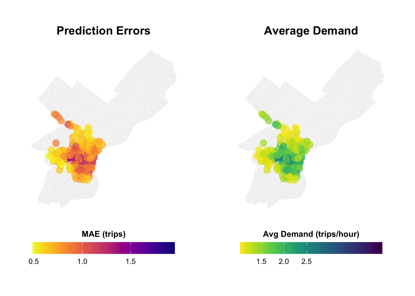
Based off this mapping, the highest prediction errors appear to be clustered in Center City, University City, and parts of Northwest Philadelphia. When comparing this to a map of Average Demand, there appears to be a relationship (where higher demand also coincides with worse model performance).

This could be because of higher demand resulting in more diverse trip origination. That is, if a lot more people are starting trips in a certain area, you may have people riding Indego for a wider variety of reasons. As a result, trip patterns might differ and the model may be unable to pick that up.

Temporal Error Analysis

Code
# MAE by time of day and day type
temporal_errors <- test %>%
  group_by(time_of_day, weekend) %>%
  summarize(
    MAE = mean(abs_error, na.rm = TRUE),
    .groups = "drop"
  ) %>%
  mutate(day_type = ifelse(weekend == 1, "Weekend", "Weekday"))

ggplot(temporal_errors, aes(x = time_of_day, y = MAE, fill = day_type)) +
  geom_col(position = "dodge") +
  scale_fill_manual(values = c("Weekday" = "#08519c", "Weekend" = "#6baed6")) +
  labs(
    title = "Prediction Errors by Time Period",
    subtitle = "When is the model struggling most?",
    x = "Time of Day",
    y = "Mean Absolute Error (trips)",
    fill = "Day Type"
  ) +
  plotTheme +
  theme(axis.text.x = element_text(angle = 45, hjust = 1))

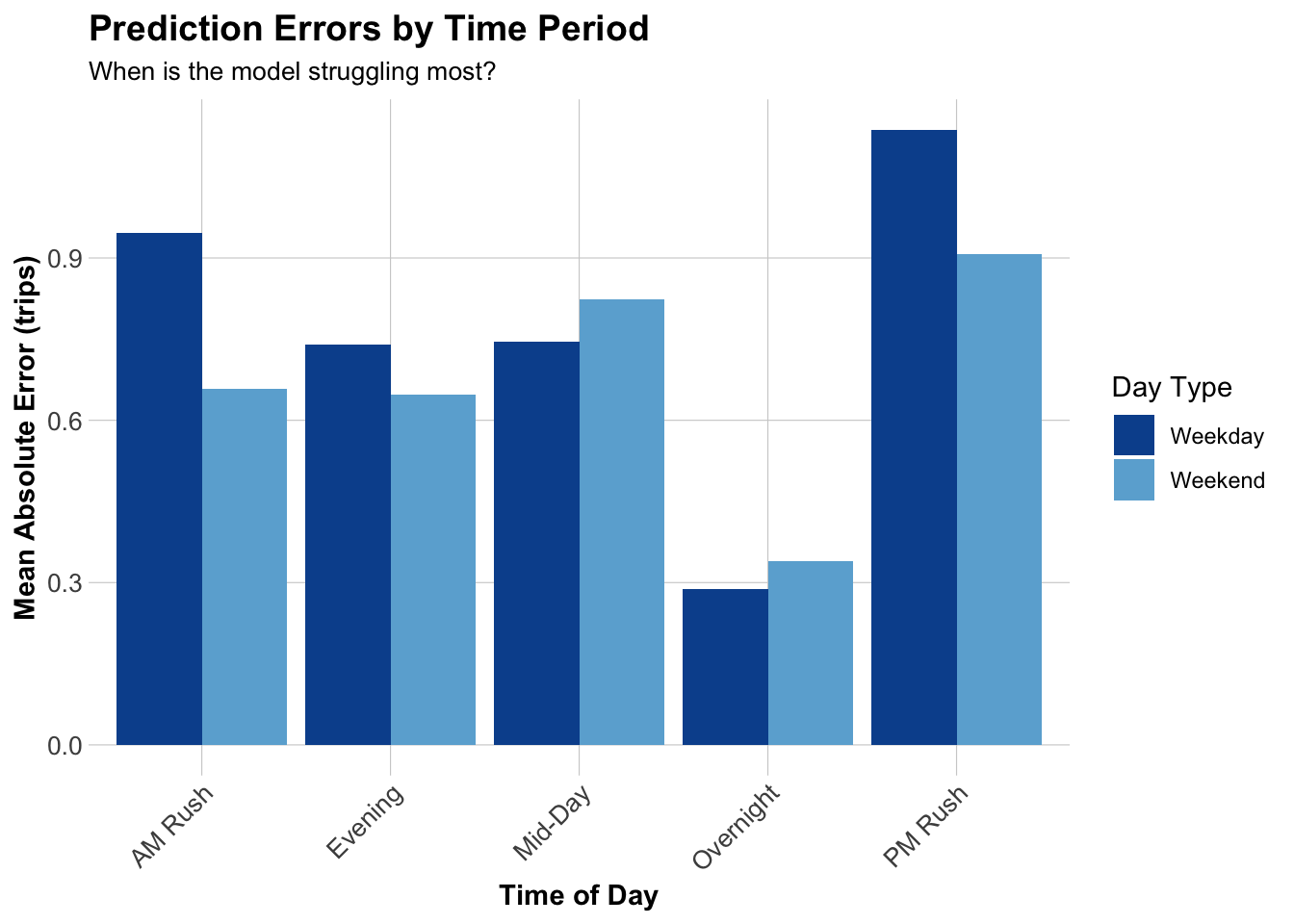
Based off of the above chart, the highest error is by far during the Weekday evening rush, followed by the Weekday morning rush. This suggests that commuting patterns may not be accounted for the model. Compared to the Q1 2025 data, the MAE here is much worse. This could suggest that commuting patterns during this chaotic time of year (return to school, evening events, etc.) may be shifting in a more granular manner than the model accounts for.

Demographic Error Analysis

Code
# Join demographic data to station errors
station_errors_demo <- station_errors %>%
  left_join(
    station_attributes %>% dplyr::select(start_station, Med_Inc, Percent_Taking_Transit, Percent_White),
    by = "start_station"
  ) %>%
  filter(!is.na(Med_Inc))

# Create plots
p1 <- ggplot(station_errors_demo, aes(x = Med_Inc, y = MAE)) +
  geom_point(alpha = 0.5, color = "#3182bd") +
  geom_smooth(method = "lm", se = FALSE, color = "red") +
  scale_x_continuous(labels = scales::dollar) +
  labs(title = "Errors vs. Median Income", x = "Median Income", y = "MAE") +
  plotTheme

p2 <- ggplot(station_errors_demo, aes(x = Percent_Taking_Transit, y = MAE)) +
  geom_point(alpha = 0.5, color = "#3182bd") +
  geom_smooth(method = "lm", se = FALSE, color = "red") +
  labs(title = "Errors vs. Transit Usage", x = "% Taking Transit", y = "MAE") +
  plotTheme

p3 <- ggplot(station_errors_demo, aes(x = Percent_White, y = MAE)) +
  geom_point(alpha = 0.5, color = "#3182bd") +
  geom_smooth(method = "lm", se = FALSE, color = "red") +
  labs(title = "Errors vs. Race", x = "% White", y = "MAE") +
  plotTheme

grid.arrange(p1, p2, p3, ncol = 2)

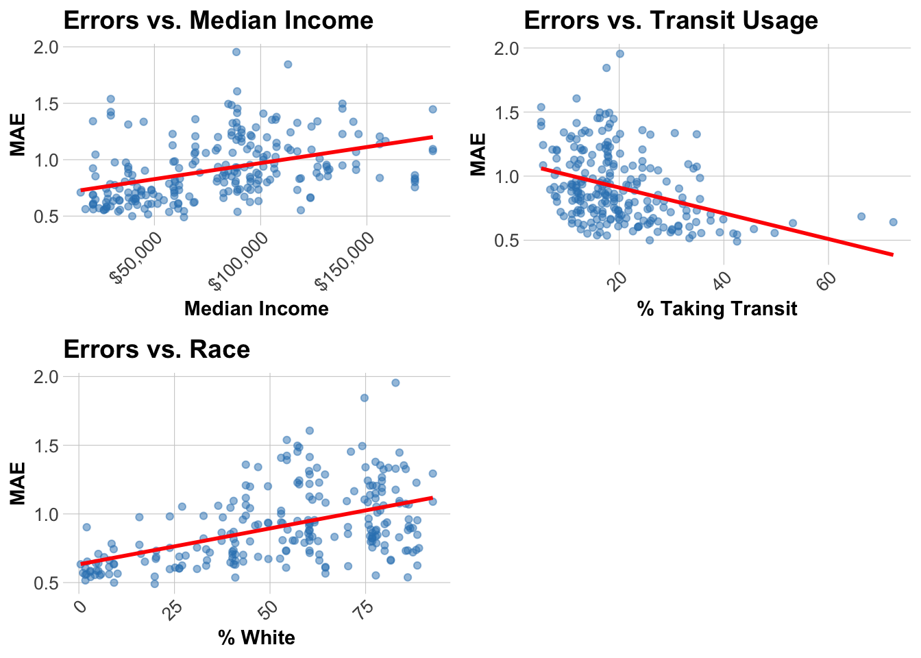
The above charts break down census demographic characteristics with respect to MAE. It appears that increasing median income and % of the tract that is white is associated with higher MAEs. There could be underlying trends with these more affluent communities that result in Indego usage patterns that are hard to predict. A less clear trend is apparent with transit usage, where a slight downward trend of MAE is associated with higher transit usage. This is less conclusive, because there are less observations in the higher transit usage tracts. The rest of the data is fairly scattered.

I suspect that the way different communities/socioeconomic groups use Indego must be accounted for in the model. Some groups may use Indego primarily for leisure or one-off travel, while others may use it for consistent commuting. There is an equity implication here because our prediction model may end up allocating resources to stations that do not need it. This is especially concerning since we showed in earlier charts that the model performs the worst during peak commuting hours.

Part 3: Feature Engineering & model improvement

Feature creation

In the below section, I am adding 3 new features to our training and testing data that will be used for an updated Model 2. First, holidays such as July 4th and Labor Day are included as a binary variable. Next, biking weather can have an impact on leisure vs commuting pattern so an aggregated binary variable called “perfect_bike_weather” is included. Finally, I found that August 26th was the earliest date that a major school reopened so this date is used to define binary variable “schools_start_opening”.

Code
train <- train %>%
  mutate(
    # Holiday indicator
    holiday = ifelse(date %in% as.Date(c("2024-07-04", "2024-09-02")), 1, 0),
    
    # Perfect biking weather
    perfect_bike_weather = ifelse(Temperature >= 60 & Temperature <= 75 & Precipitation == 0, 1, 0),
    
    # The earliest date that schools start opening in Philly (between UPenn, Drexel, Temple, and Philly Public Schools)
    schools_start_opening = ifelse(interval60 >= as.POSIXct("2024-08-26"), 1, 0)
  )

test <- test %>%
  mutate(
    holiday = ifelse(date %in% as.Date(c("2024-07-04", "2024-09-02")), 1, 0),
    
    perfect_bike_weather = ifelse(Temperature >= 60 & Temperature <= 75 & Precipitation == 0, 1, 0),
    
    schools_start_opening = ifelse(interval60 >= as.POSIXct("2024-08-26"), 1, 0)
  )

Enhanced Model Creation and Comparison

Below, we create a model based on Model 2 but with the 3 new features included.

Code
model2_new <- lm(
  Trip_Count ~ as.factor(hour) + dotw_simple + Temperature + Precipitation +
    lag1Hour + lag3Hours + lag1day +
    holiday + perfect_bike_weather + schools_start_opening,
  data = train
)

summary(model2_new)

Call:
lm(formula = Trip_Count ~ as.factor(hour) + dotw_simple + Temperature + 
    Precipitation + lag1Hour + lag3Hours + lag1day + holiday + 
    perfect_bike_weather + schools_start_opening, data = train)

Residuals:
    Min      1Q  Median      3Q     Max 
-7.7870 -0.4916 -0.1368  0.1959 20.2900 

Coefficients:
                        Estimate Std. Error t value             Pr(>|t|)    
(Intercept)           -0.0001819  0.0312853  -0.006             0.995360    
as.factor(hour)1      -0.0308293  0.0109516  -2.815             0.004877 ** 
as.factor(hour)2      -0.0206977  0.0111578  -1.855             0.063596 .  
as.factor(hour)3      -0.0451866  0.0114966  -3.930 0.000084810479935988 ***
as.factor(hour)4      -0.0262611  0.0113217  -2.320             0.020366 *  
as.factor(hour)5       0.0913578  0.0111951   8.161 0.000000000000000335 ***
as.factor(hour)6       0.2882684  0.0113386  25.424 < 0.0000000000000002 ***
as.factor(hour)7       0.4445139  0.0113420  39.192 < 0.0000000000000002 ***
as.factor(hour)8       0.6869282  0.0113434  60.558 < 0.0000000000000002 ***
as.factor(hour)9       0.3004831  0.0114281  26.293 < 0.0000000000000002 ***
as.factor(hour)10      0.2543072  0.0112145  22.677 < 0.0000000000000002 ***
as.factor(hour)11      0.2780552  0.0113687  24.458 < 0.0000000000000002 ***
as.factor(hour)12      0.4029540  0.0112767  35.733 < 0.0000000000000002 ***
as.factor(hour)13      0.3696691  0.0110812  33.360 < 0.0000000000000002 ***
as.factor(hour)14      0.4138605  0.0111255  37.199 < 0.0000000000000002 ***
as.factor(hour)15      0.4482541  0.0110501  40.566 < 0.0000000000000002 ***
as.factor(hour)16      0.6126921  0.0113767  53.855 < 0.0000000000000002 ***
as.factor(hour)17      0.8666137  0.0114940  75.397 < 0.0000000000000002 ***
as.factor(hour)18      0.4924912  0.0115943  42.477 < 0.0000000000000002 ***
as.factor(hour)19      0.3784903  0.0113875  33.237 < 0.0000000000000002 ***
as.factor(hour)20      0.2309382  0.0110230  20.951 < 0.0000000000000002 ***
as.factor(hour)21      0.1350206  0.0110838  12.182 < 0.0000000000000002 ***
as.factor(hour)22      0.1439564  0.0108079  13.320 < 0.0000000000000002 ***
as.factor(hour)23      0.0582946  0.0114474   5.092 0.000000353754764879 ***
dotw_simple2           0.0209249  0.0063333   3.304             0.000953 ***
dotw_simple3           0.0134653  0.0062161   2.166             0.030297 *  
dotw_simple4          -0.0262262  0.0064166  -4.087 0.000043660333745859 ***
dotw_simple5          -0.0332034  0.0062229  -5.336 0.000000095220493801 ***
dotw_simple6          -0.0377046  0.0062738  -6.010 0.000000001858957165 ***
dotw_simple7          -0.0575069  0.0062055  -9.267 < 0.0000000000000002 ***
Temperature           -0.0002638  0.0003673  -0.718             0.472697    
Precipitation          0.0865538  0.0284900   3.038             0.002381 ** 
lag1Hour               0.3766745  0.0014351 262.481 < 0.0000000000000002 ***
lag3Hours              0.1280059  0.0014107  90.741 < 0.0000000000000002 ***
lag1day                0.1449832  0.0013185 109.964 < 0.0000000000000002 ***
holiday               -0.0298609  0.0147311  -2.027             0.042657 *  
perfect_bike_weather   0.0216988  0.0050730   4.277 0.000018920436050917 ***
schools_start_opening  0.0047859  0.0055443   0.863             0.388022    
---
Signif. codes:  0 '***' 0.001 '**' 0.01 '*' 0.05 '.' 0.1 ' ' 1

Residual standard error: 1.046 on 426957 degrees of freedom
Multiple R-squared:  0.3307,    Adjusted R-squared:  0.3306 
F-statistic:  5702 on 37 and 426957 DF,  p-value: < 0.00000000000000022

Below, we compare the MAE between Model 2 and the Enhanced Model 2.

Code
test <- test %>%
  mutate(
    pred2_new = predict(model2_new, newdata = test)
  )

mae_old <- mean(abs(test$Trip_Count - test$pred2), na.rm = TRUE)
mae_new <- mean(abs(test$Trip_Count - test$pred2_new), na.rm = TRUE)

cat("Old MAE (Model 2):", round(mae_old, 3), "\n")
Old MAE (Model 2): 0.69 
Code
cat("New MAE (Model 2 + 3 features):", round(mae_new, 3), "\n")
New MAE (Model 2 + 3 features): 0.691 

Based on these results, it turns out that the 3 additional features reduced model performance from the simpler model. On the side, I messed around with the 3 additional features (removing and keeping various combinations). None of the combinations resulted in an MAE that was less than the original Model 2!

Poisson Model for Count Data

Code
library(MASS)

# Poisson Model 2: Original
poisson_model_orig <- glm(
  Trip_Count ~ as.factor(hour) + dotw_simple + Temperature + Precipitation +
    lag1Hour + lag3Hours + lag1day,
  family = poisson(link = "log"),
  data = train
)

# Poisson Model 2: Enhanced with new features
poisson_model_new <- glm(
  Trip_Count ~ as.factor(hour) + dotw_simple + Temperature + Precipitation +
    lag1Hour + lag3Hours + lag1day + perfect_bike_weather + schools_start_opening,
  family = poisson(link = "log"),
  data = train
)
Code
test <- test %>%
  mutate(
    pred_poisson_orig = predict(poisson_model_orig, newdata = test, type = "response"),
    pred_poisson_new  = predict(poisson_model_new, newdata = test, type = "response")
  )

mae_poisson_orig <- mean(abs(test$Trip_Count - test$pred_poisson_orig), na.rm = TRUE)
mae_poisson_new  <- mean(abs(test$Trip_Count - test$pred_poisson_new), na.rm = TRUE)

cat("MAE - Poisson Original Model 2:", round(mae_poisson_orig,2), "\n")
MAE - Poisson Original Model 2: 0.74 
Code
cat("MAE - Poisson Enhanced Model 2:", round(mae_poisson_new,2), "\n")
MAE - Poisson Enhanced Model 2: 0.74 

Running Poisson did not improve model fit, for either the original Model 2 or the Enhanced Model 2.

Part 4: Critical Reflection

  1. Operational implications:

It is clear that the MAE is not good enough for Indego usage. First, the MAE for this quarter is worse than for Q1 2025. This suggests that there is variability over the course of the year that the model must account for. We also showed that demographic data is associated with higher or lower levels of MAE in the model. Next, all models regardless of time of year performed worse in parts of Philadelphia with the highest Indego demand. This alone defeats the purpose of ensuring Indego availability at stations.

My recommendation is further adjusting this model, especially to account for shifts in morning and evening commuting patterns. Once this is done, the model can be deployed for use. MAE is not a catch-all indicator, since a higher MAE might be acceptable during lower volume but higher variation times of Indego use. Alas, this is not the case with the models in this report, with worse performance during peak hours.

  1. Equity considerations:

The model could impact equity by not stocking bikes at stations where users who rely on them for commuting may be. This is reflected in the worse MAE for peak hours during weekdays. One could argue that commuting hours are more critical than conventional recreational hours for model accuracy. Missing Indego bikes during these times could hinder the ability of someone to get to work or go home.

  1. Model limitations:

With more time, I would explore how neighborhoods effect Indego usage patterns (casual vs commuting), and how events throughout Philadelphia impact ridership. These are not entirely accounted for in the models in this report.