Assignment 4: Spatial Predictive Analysis

Chicago 311 Data

Setup

# Set options
options(scipen = 999)  # No scientific notation
set.seed(5080)         # Reproducibility

# Packages
library(tidyverse)      # Data manipulation
library(sf)             # Spatial operations
library(here)           # Relative file paths
library(viridis)        # Color scales
library(terra)          # Raster operations (replaces 'raster')
library(spdep)          # Spatial dependence
library(FNN)            # Fast nearest neighbors
library(MASS)           # Negative binomial regression
library(patchwork)      # Plot composition (replaces grid/gridExtra)
library(knitr)          # Tables
library(kableExtra)     # Table formatting
library(classInt)       # Classification intervals

# Spatstat split into sub-packages
library(spatstat.geom)    # Spatial geometries
library(spatstat.explore) # Spatial exploration/KDE

# Set options
options(scipen = 999)  # No scientific notation
set.seed(5080)         # Reproducibility

# Create consistent theme for visualizations
theme_crime <- function(base_size = 11) {
  theme_minimal(base_size = base_size) +
    theme(
      plot.title = element_text(face = "bold", size = base_size + 1),
      plot.subtitle = element_text(color = "gray30", size = base_size - 1),
      legend.position = "right",
      panel.grid.minor = element_blank(),
      axis.text = element_blank(),
      axis.title = element_blank()
    )
}

# Set as default
theme_set(theme_crime())

Data Loading & Exploration

First, some contextual boundaries are being loaded. We have Chicago Police District boundaries, Police Beats (smaller than districts), and the City boundary itself.

# Load police districts (used for spatial cross-validation)
policeDistricts <- 
  st_read("https://data.cityofchicago.org/api/geospatial/24zt-jpfn?method=export&format=GeoJSON", quiet = TRUE) %>%
  st_transform('ESRI:102271', quiet = TRUE) %>%
  dplyr::select(District = dist_num)

# Load police beats (smaller administrative units)
policeBeats <- 
  st_read("https://data.cityofchicago.org/api/geospatial/n9it-hstw?method=export&format=GeoJSON", quiet = TRUE) %>%
  st_transform('ESRI:102271', quiet = TRUE) %>%
  dplyr::select(Beat = beat_num)

# Load Chicago boundary
chicagoBoundary <- 
  st_read("https://raw.githubusercontent.com/urbanSpatial/Public-Policy-Analytics-Landing/master/DATA/Chapter5/chicagoBoundary.geojson", quiet = TRUE) %>%
  st_transform('ESRI:102271', quiet = TRUE)

NoteCoordinate Reference System

We’re using ESRI:102271 (Illinois State Plane East, NAD83, US Feet). This is appropriate for Chicago because:

• It minimizes distortion in this region
• Uses feet (common in US planning)
• Allows accurate distance calculations

Eventually, we will create predictive models for burglaries. Here, we load Chicago Burglary data.

# Load from provided data file (downloaded from Chicago open data portal)
burglaries <- st_read("./data/burglaries.shp", quiet = TRUE) %>% 
  st_transform('ESRI:102271', quiet = TRUE)

cat(glue::glue("
### Burglary Data Check

**✓ Loaded burglary data**

- **Number of burglaries:** {nrow(burglaries)}
- **CRS:** {st_crs(burglaries)$input}
- **Date range:** {min(burglaries$date, na.rm = TRUE)} to {max(burglaries$date, na.rm = TRUE)}
"))

### Burglary Data Check

**✓ Loaded burglary data**

- **Number of burglaries:** 7482
- **CRS:** ESRI:102271
- **Date range:** Inf to -Inf

One predictor that will be explored is 311 Data focused on street light outages. Specifically, this data contains points where single street light outages were reported. I chose this feature mostly out of curiosity. Vacant buildings, abandoned cars, etc are examples of physcial properties that can be connected to crimes, but street light outages on a surface level seem less connected.

street_lights <- read_csv("./data/311_Single_Street_Light_Out.csv")%>%
  filter(!is.na(Latitude), !is.na(Longitude)) %>%
  st_as_sf(coords = c("Longitude", "Latitude"), crs = 4326) %>%
  st_transform('ESRI:102271')

Visualizing Single Street Light Outages from 311 Data

Simple Choropleth Map

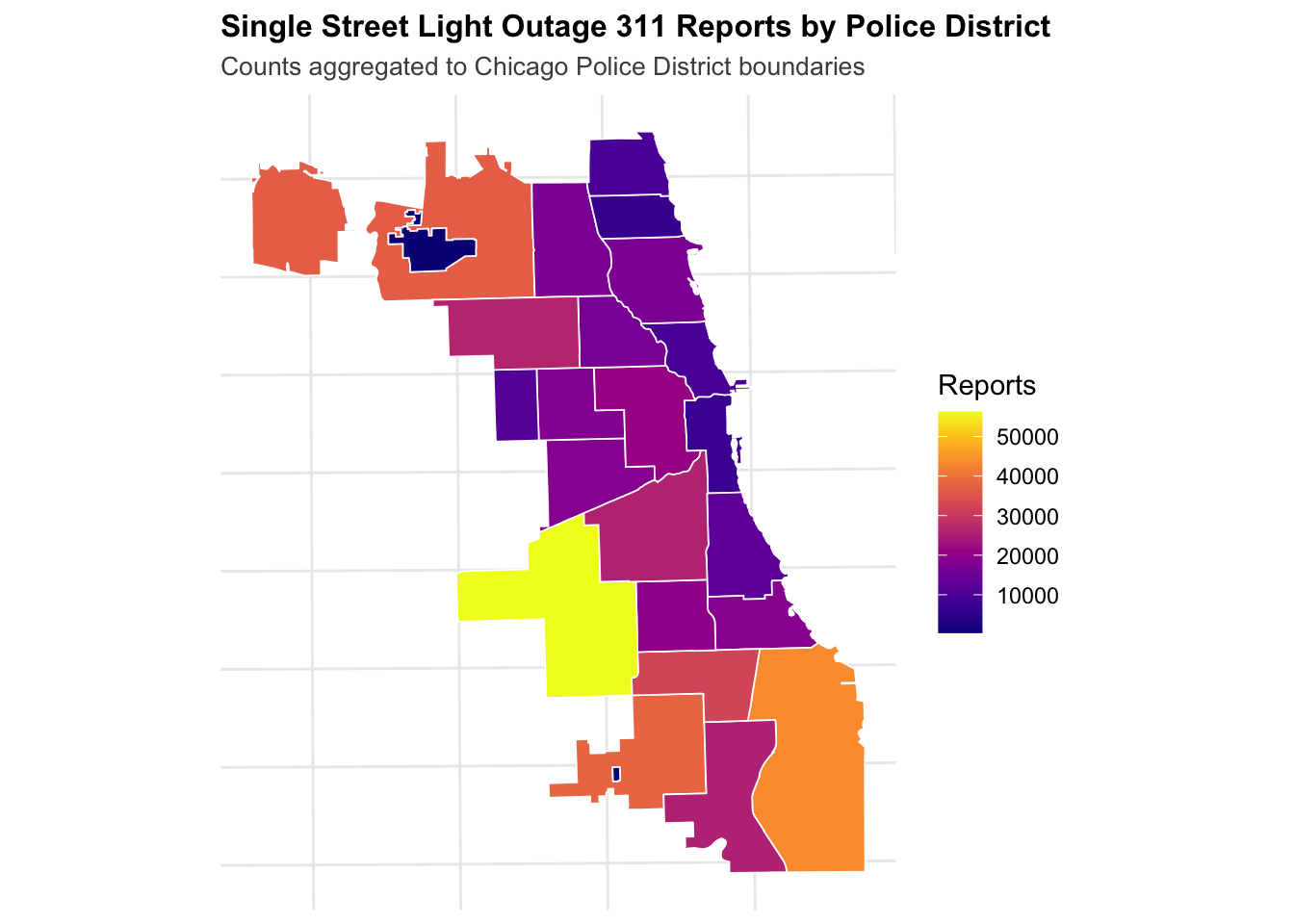
First, I want to visualize the single lights outage data with a choropleth map using Chicago PD boundaries. This will not be the most insightful visualization, but I want to get an idea of the data before proceeding with other methods.

# Aggregate street lights out by police district
lights_by_district <- 
  policeDistricts %>%
  st_join(street_lights) %>%
  count(District, name = "lights_out")

# Choropleth map
ggplot() +
  geom_sf(data = lights_by_district, 
          aes(fill = lights_out), 
          color = "white", size = 0.3) +
  scale_fill_viridis(option = "plasma", direction = 1) +
  labs(
    title = "Single Street Light Outage 311 Reports by Police District",
    subtitle = "Counts aggregated to Chicago Police District boundaries",
    fill = "Reports"
  ) +
  theme_crime()

Here, we see the greatest number of reports in southern, south-western, and north-western Police Districts, and lower numbers in central and northern ones.

Fishnet Grid and Visualization

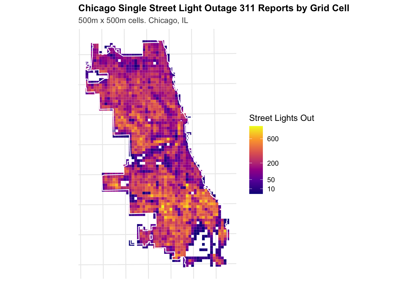
As stated previously, arbitrary boundaries like police districts make analysis more complicated and less reliable for real-world conditions. Here, we use a 500m x 500m “fishnet” over the City of Chicago, where each grid cell has aggregated counts for 311 Single Light Outage complaints.

# Create a 500mx500m fishnet
fishnet_lights <- st_make_grid(
  chicagoBoundary,
  cellsize = 500,
  square = TRUE
) %>%
  st_sf() %>%
  mutate(uniqueID = row_number())

# Aggregate burglaries to the same fishnet grid
burglaries_fishnet <- st_join(burglaries, fishnet_lights, join = st_within) %>%
  st_drop_geometry() %>%
  group_by(uniqueID) %>%
  summarize(countBurglaries = n())

# Join burglary counts to fishnet
fishnet_lights <- fishnet_lights %>%
  left_join(burglaries_fishnet, by = "uniqueID") %>%
  mutate(countBurglaries = replace_na(countBurglaries, 0))

# Spatial join: assign each street light to a grid cell
lights_fishnet <- st_join(street_lights, fishnet_lights, join = st_within) %>%
  st_drop_geometry() %>%
  group_by(uniqueID) %>%
  summarize(countLights = n())

# Join back to fishnet (cells with zero lights will be NA → convert to 0)
fishnet_lights <- fishnet_lights %>%
  left_join(lights_fishnet, by = "uniqueID") %>%
  mutate(countLights = replace_na(countLights, 0))

# Finally, I want to filter out cells with zero counts, as that will mess wth future analysis
fishnet_lights <- fishnet_lights %>%
  filter(countLights > 0)

ggplot() +
  geom_sf(data = fishnet_lights, aes(fill = countLights), color = NA) +
  geom_sf(data = chicagoBoundary, fill = NA, color = "white", linewidth = 0.5) +
  scale_fill_viridis_c(
    name = "Street Lights Out",
    option = "plasma",
    trans = "sqrt",
    breaks = c(0, 10, 50, 200, 600)
  ) +
  labs(
    title = "Chicago Single Street Light Outage 311 Reports by Grid Cell",
    subtitle = "500m x 500m cells. Chicago, IL"
  ) +
  theme_crime()

Here, the fishnet grid provides a more granular view of street light outages across the city. In the southernmost police district—which the choropleth map previously suggested had the highest number of 311 complaints—we now see substantial variation: much of the district has relatively few complaints, while hotspots appear in the northern portions. Similarly, northern and western Chicago contains concentrated pockets of higher complaint activity that are obscured when aggregated at the district level.

We can explore this spatial variation in the following section.

Spatial Feature Development

k-Nearest Neighbor Features

# 3.2 Nearest Neighbor Features
# Coordinates
fishnet_coords <- st_coordinates(st_centroid(fishnet_lights))
lights_coords <- st_coordinates(street_lights)

# kNN distances
nn_result <- get.knnx(lights_coords, fishnet_coords, k = 3)

# Add to fishnet
fishnet_lights <- fishnet_lights %>%
  mutate(lights_out_nn = rowMeans(nn_result$nn.dist))

summary(fishnet_lights$lights_out_nn)

   Min. 1st Qu.  Median    Mean 3rd Qu.    Max. 
   1.89   29.32   45.95   66.50   75.31  625.47 

# Function to calculate Local Moran's I
calculate_local_morans <- function(data, variable, k = 3) {
  
  # Create spatial weights
  coords <- st_coordinates(st_centroid(data))
  neighbors <- knn2nb(knearneigh(coords, k = k))
  weights <- nb2listw(neighbors, style = "W", zero.policy = TRUE)
  
  # Calculate Local Moran's I
  local_moran <- localmoran(data[[variable]], weights)
  
  # Classify clusters
  mean_val <- mean(data[[variable]], na.rm = TRUE)
  
  data %>%
    mutate(
      local_i = local_moran[, 1],
      p_value = local_moran[, 5],
      is_significant = p_value < 0.05,
      
      moran_class = case_when(
        !is_significant ~ "Not Significant",
        local_i > 0 & .data[[variable]] > mean_val ~ "High-High",
        local_i > 0 & .data[[variable]] <= mean_val ~ "Low-Low",
        local_i < 0 & .data[[variable]] > mean_val ~ "High-Low",
        local_i < 0 & .data[[variable]] <= mean_val ~ "Low-High",
        TRUE ~ "Not Significant"
      )
    )
}

fishnet_lights_morans <- calculate_local_morans(fishnet_lights, "countLights", k = 5)

# Visualize clusters
ggplot() +
  geom_sf(data = fishnet_lights_morans, aes(fill = moran_class), color = NA) +
  geom_sf(data = chicagoBoundary, fill = NA, color = "black", linewidth = 0.4) +
  scale_fill_manual(
    values = c(
      "High-High" = "#d7191c",
      "High-Low" = "#fdae61",
      "Low-High" = "#abd9e9",
      "Low-Low" = "#2c7bb6",
      "Not Significant" = "gray90"
    ),
    name = "Cluster Type"
  ) +
  labs(
    title = "Local Moran's I: Street Light Outage Clusters",
    subtitle = "High-High = Hot spots of outages; k=3 neighbors"
  ) +
  theme_crime()

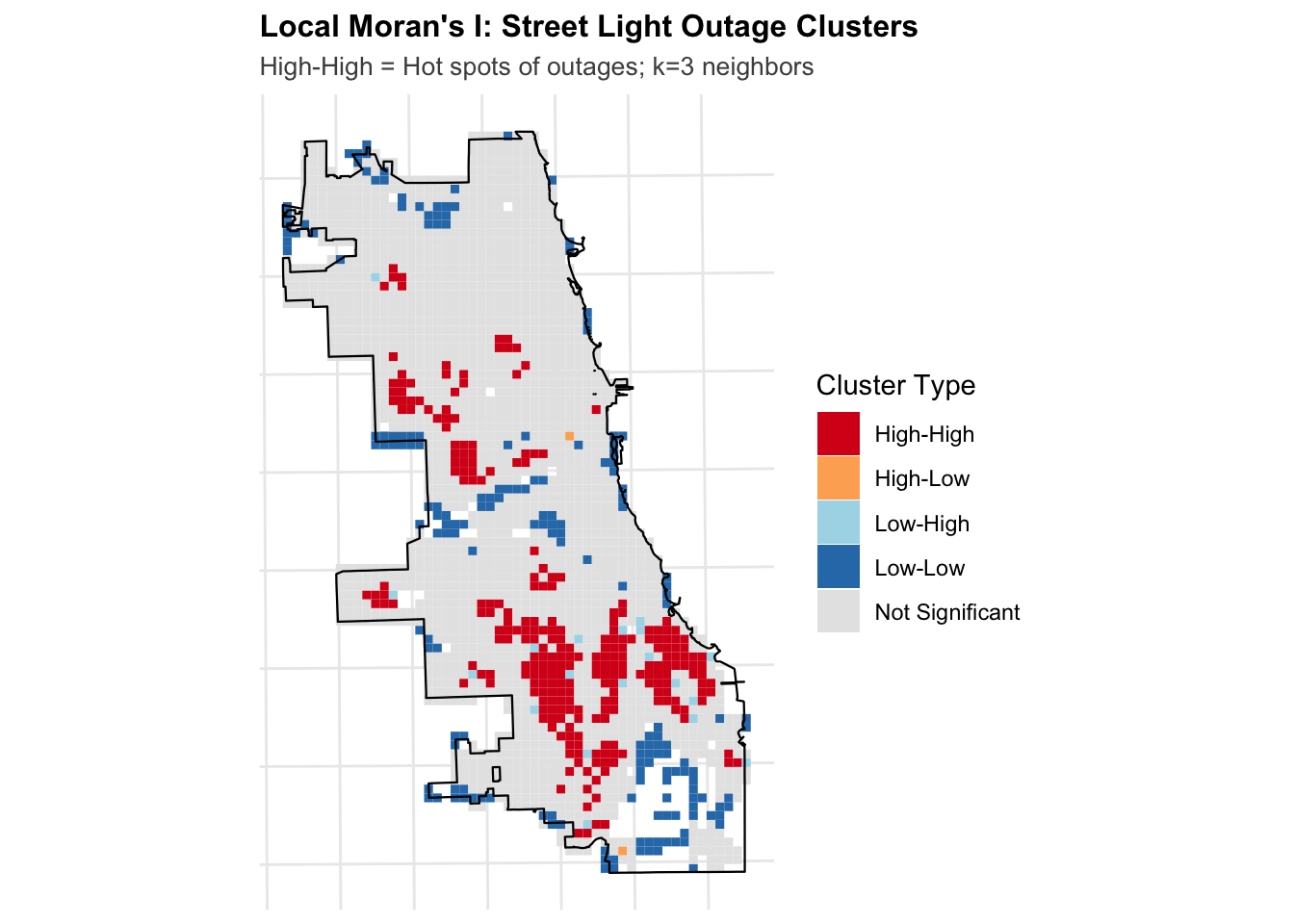
The calculate_local_morans function was provided in class. The function wraps R’s localmoran() to automate spatial weight creation and classify cells into interpretable cluster types (High-High, Low-Low, etc.), which localmoran() doesn’t provide—it only returns raw statistics.

The Local Moran’s I results confirm clustering visible in the fishnet map, with High-High clusters concentrated in South Chicago where high outage counts are surrounded by other high-count cells. Areas of High-High and Low-Low cells can be considered as hotspots and coldspots respectively. This can be a useful parameter for the remainder of this report, so it is calculated below. In addition, we can calculate distances between every cell and the nearest hot and cold spots.

# Get centroids of "High-High" cells (hot spots)
hotspots <- fishnet_lights_morans %>%
  filter(moran_class == "High-High") %>%
  st_centroid()

# Calculate distance from each cell to nearest hot spot
if (nrow(hotspots) > 0) {
  fishnet_lights_morans <- fishnet_lights_morans %>%
    mutate(
      dist_to_hotspot = as.numeric(
        st_distance(st_centroid(fishnet_lights_morans), hotspots %>% st_union())
      )
    )
  
  cat("✓ Calculated distance to single light outage hot spots\n")
  cat("  - Number of hot spot cells:", nrow(hotspots), "\n")
} else {
  fishnet_lights_morans <- fishnet_lights_morans %>%
    mutate(dist_to_hotspot = 0)
  cat("⚠ No significant hot spots found\n")
}

✓ Calculated distance to single light outage hot spots
  - Number of hot spot cells: 260 

# Get centroids of "Low-Low" cells (cold spots)
coldspots <- fishnet_lights_morans %>%
  filter(moran_class == "Low-Low") %>%
  st_centroid()

# Calculate distance from each cell to nearest cold spot
if (nrow(coldspots) > 0) {
  fishnet_lights_morans <- fishnet_lights_morans %>%
    mutate(
      dist_to_coldspot = as.numeric(
        st_distance(st_centroid(fishnet_lights_morans), coldspots %>% st_union())
      )
    )
  
  cat("✓ Calculated distance to single light outage cold spots\n")
  cat("  - Number of cold spot cells:", nrow(coldspots), "\n")
} else {
  fishnet_lights_morans <- fishnet_lights_morans %>%
    mutate(dist_to_coldspot = 0)
  cat("⚠ No significant cold spots found\n")
}

✓ Calculated distance to single light outage cold spots
  - Number of cold spot cells: 180 

# Summary statistics for distance features
tibble(
  Metric = c("Min", "Q1", "Median", "Mean", "Q3", "Max"),
  `Distance to Hot Spots` = summary(fishnet_lights_morans$dist_to_hotspot),
  `Distance to Cold Spots` = summary(fishnet_lights_morans$dist_to_coldspot)
) %>%
  kable(
    caption = "Summary Statistics: Distance to Hot Spots and Cold Spots (feet)",
    digits = 0,
    format.args = list(big.mark = ",")
  ) %>%
  kable_styling(bootstrap_options = c("striped", "hover", "condensed"))

Summary Statistics: Distance to Hot Spots and Cold Spots (feet)

Metric	Distance to Hot Spots	Distance to Cold Spots
Min	0.0	0
Q1	707.1	1,000
Median	1,581.1	1,803
Mean	2,200.3	2,116
Q3	3,041.4	3,041
Max	10,965.9	6,265

Count Regression Models

Poisson Regression

Since light outages are simple counts, we can first try to create a Poisson Regression Model.

# Join district information to fishnet
fishnet_lights_morans <- st_join(
  fishnet_lights_morans,
  policeDistricts,
  join = st_within,
  left = TRUE
)

# Filter using base R subsetting
fishnet_lights_morans <- fishnet_lights_morans[!is.na(fishnet_lights_morans$District), ]

cat("✓ Joined police districts\n")

✓ Joined police districts

cat("  - Districts:", length(unique(fishnet_lights_morans$District)), "\n")

  - Districts: 22 

cat("  - Cells:", nrow(fishnet_lights_morans), "\n")

  - Cells: 1611 

# Fit Poisson regression predicting BURGLARIES
model_poisson_burglary <- glm(
  countBurglaries ~ countLights + lights_out_nn + dist_to_hotspot + dist_to_coldspot,
  data = fishnet_lights_morans,
  family = "poisson"
)

# Summary
summary(model_poisson_burglary)

Call:
glm(formula = countBurglaries ~ countLights + lights_out_nn + 
    dist_to_hotspot + dist_to_coldspot, family = "poisson", data = fishnet_lights_morans)

Coefficients:
                     Estimate   Std. Error z value             Pr(>|z|)    
(Intercept)       1.065585574  0.057115217  18.657 < 0.0000000000000002 ***
countLights       0.001557601  0.000103340  15.073 < 0.0000000000000002 ***
lights_out_nn    -0.006864476  0.000500108 -13.726 < 0.0000000000000002 ***
dist_to_hotspot  -0.000064158  0.000008971  -7.151    0.000000000000859 ***
dist_to_coldspot  0.000100867  0.000009376  10.758 < 0.0000000000000002 ***
---
Signif. codes:  0 '***' 0.001 '**' 0.01 '*' 0.05 '.' 0.1 ' ' 1

(Dispersion parameter for poisson family taken to be 1)

    Null deviance: 6016.5  on 1610  degrees of freedom
Residual deviance: 4411.3  on 1606  degrees of freedom
AIC: 8477.6

Number of Fisher Scoring iterations: 5

# Calculate dispersion parameter
dispersion <- sum(residuals(model_poisson_burglary, type = "pearson")^2) / 
              model_poisson_burglary$df.residual

cat("Dispersion parameter:", round(dispersion, 2), "\n")

Dispersion parameter: 2.96 

cat("Rule of thumb: >1.5 suggests overdispersion\n")

Rule of thumb: >1.5 suggests overdispersion

if (dispersion > 1.5) {
  cat("⚠ Overdispersion detected! Consider Negative Binomial model.\n")
} else {
  cat("✓ Dispersion looks okay for Poisson model.\n")
}

⚠ Overdispersion detected! Consider Negative Binomial model.

The Poisson regression shows that all four street light features are statistically significant predictors of burglary counts. Areas with more light outages tend to have more burglaries, and being closer to outage hotspots is associated with higher counts of burglaries as well. However, the high residual deviance confirms overdispersion, which is why we can try the Negative Binomial model instead.

Negative Binomial

# Fit Negative Binomial model predicting BURGLARIES
model_nb_burglary <- glm.nb(
  countBurglaries ~ countLights + lights_out_nn + dist_to_hotspot + dist_to_coldspot,
  data = fishnet_lights_morans
)

# Summary
summary(model_nb_burglary)

Call:
glm.nb(formula = countBurglaries ~ countLights + lights_out_nn + 
    dist_to_hotspot + dist_to_coldspot, data = fishnet_lights_morans, 
    init.theta = 2.007649347, link = log)

Coefficients:
                    Estimate  Std. Error z value             Pr(>|z|)    
(Intercept)       0.91119504  0.09865200   9.236 < 0.0000000000000002 ***
countLights       0.00197739  0.00019753  10.011 < 0.0000000000000002 ***
lights_out_nn    -0.00797075  0.00077198 -10.325 < 0.0000000000000002 ***
dist_to_hotspot  -0.00004062  0.00001388  -2.925              0.00344 ** 
dist_to_coldspot  0.00012039  0.00001698   7.092     0.00000000000132 ***
---
Signif. codes:  0 '***' 0.001 '**' 0.01 '*' 0.05 '.' 0.1 ' ' 1

(Dispersion parameter for Negative Binomial(2.0076) family taken to be 1)

    Null deviance: 2445.8  on 1610  degrees of freedom
Residual deviance: 1779.9  on 1606  degrees of freedom
AIC: 7295.1

Number of Fisher Scoring iterations: 1

              Theta:  2.008 
          Std. Err.:  0.121 

 2 x log-likelihood:  -7283.051 

# Compare models
cat("\n### Model Comparison (AIC - lower is better):\n")

### Model Comparison (AIC - lower is better):

cat("Poisson AIC:", round(AIC(model_poisson_burglary), 1), "\n")

Poisson AIC: 8477.6 

cat("Negative Binomial AIC:", round(AIC(model_nb_burglary), 1), "\n")

Negative Binomial AIC: 7295.1 

The Negative Binomial model shows all predictors remain significant, with the same relationships: more light outages and closer proximity to hotspots are associated with higher burglary counts. The much lower AIC (7,295 vs 8,477.6) confirms this model performs better than Poisson.

Spatial Cross Validation

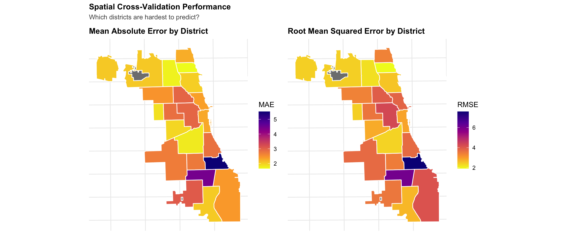
Standard cross-validation randomly splits data, but with spatial data this means training on cells directly adjacent to test cells (spatial information leakage). Leave-One-Group-Out (LOGO) Cross-Validation addresses this by training on all police districts except one, then testing on the held-out district.

# Create clean modeling dataset
fishnet_model <- fishnet_lights_morans %>%
  st_drop_geometry() %>%
  dplyr::select(
    uniqueID,
    District,
    countBurglaries,
    countLights,
    lights_out_nn,
    dist_to_hotspot,
    dist_to_coldspot
  ) %>%
  na.omit()  # Remove any remaining NAs

cat("  - Observations:", nrow(fishnet_model), "\n")

  - Observations: 1611 

cat("  - Districts:", length(unique(fishnet_model$District)), "\n")

  - Districts: 22 

# Get unique districts
districts <- unique(fishnet_model$District)
cv_results <- tibble()

cat("Running LOGO Cross-Validation...\n")

Running LOGO Cross-Validation...

for (i in seq_along(districts)) {
  
  test_district <- districts[i]
  
  # Split data
  train_data <- fishnet_model %>% filter(District != test_district)
  test_data <- fishnet_model %>% filter(District == test_district)
  
  # Fit model on training data
  model_cv <- glm.nb(
    countBurglaries ~ countLights + lights_out_nn + 
      dist_to_hotspot + dist_to_coldspot,
    data = train_data
  )
  
  # Predict on test data
  test_data <- test_data %>%
    mutate(
      prediction = predict(model_cv, test_data, type = "response")
    )
  
  # Calculate metrics
  mae <- mean(abs(test_data$countBurglaries - test_data$prediction))
  rmse <- sqrt(mean((test_data$countBurglaries - test_data$prediction)^2))
  
  # Store results
  cv_results <- bind_rows(
    cv_results,
    tibble(
      fold = i,
      test_district = test_district,
      n_test = nrow(test_data),
      mae = mae,
      rmse = rmse
    )
  )
  
  cat("  Fold", i, "/", length(districts), "- District", test_district, 
      "- MAE:", round(mae, 2), "\n")
}

  Fold 1 / 22 - District 5 - MAE: 2.03 
  Fold 2 / 22 - District 4 - MAE: 2.41 
  Fold 3 / 22 - District 22 - MAE: 3.06 
  Fold 4 / 22 - District 6 - MAE: 4.44 
  Fold 5 / 22 - District 8 - MAE: 2.69 
  Fold 6 / 22 - District 7 - MAE: 2.73 
  Fold 7 / 22 - District 3 - MAE: 5.53 
  Fold 8 / 22 - District 2 - MAE: 2.82 
  Fold 9 / 22 - District 9 - MAE: 1.79 
  Fold 10 / 22 - District 10 - MAE: 1.94 
  Fold 11 / 22 - District 1 - MAE: 2.28 
  Fold 12 / 22 - District 12 - MAE: 2.93 
  Fold 13 / 22 - District 15 - MAE: 1.87 
  Fold 14 / 22 - District 11 - MAE: 2.84 
  Fold 15 / 22 - District 18 - MAE: 2.36 
  Fold 16 / 22 - District 25 - MAE: 2.45 
  Fold 17 / 22 - District 14 - MAE: 2.94 
  Fold 18 / 22 - District 19 - MAE: 2 
  Fold 19 / 22 - District 16 - MAE: 2.05 
  Fold 20 / 22 - District 17 - MAE: 1.74 
  Fold 21 / 22 - District 20 - MAE: 1.66 
  Fold 22 / 22 - District 24 - MAE: 2.25 

# Overall results
cat("\n✓ Cross-Validation Complete\n")

✓ Cross-Validation Complete

cat("Mean MAE:", round(mean(cv_results$mae), 2), "\n")

Mean MAE: 2.58 

cat("Mean RMSE:", round(mean(cv_results$rmse), 2), "\n")

Mean RMSE: 3.49 

tibble(
  Metric = c("Mean MAE", "Mean RMSE", "Std Dev MAE", "Std Dev RMSE"),
  Value = c(
    mean(cv_results$mae),
    mean(cv_results$rmse),
    sd(cv_results$mae),
    sd(cv_results$rmse)
  )
) %>%
  kable(
    digits = 2,
    caption = "Overall Cross-Validation Performance",
    format.args = list(big.mark = ",")
  ) %>%
  kable_styling(bootstrap_options = c("striped", "hover", "condensed"))

Overall Cross-Validation Performance

Metric	Value
Mean MAE	2.58
Mean RMSE	3.49
Std Dev MAE	0.90
Std Dev RMSE	1.29

# Join CV results to police districts for mapping
districts_cv <- policeDistricts %>%
  left_join(cv_results, by = c("District" = "test_district"))

# Map MAE by district
p1 <- ggplot() +
  geom_sf(data = districts_cv, aes(fill = mae), color = "white", linewidth = 0.5) +
  scale_fill_viridis_c(
    name = "MAE",
    option = "plasma",
    direction = -1
  ) +
  labs(
    title = "Mean Absolute Error by District"
  ) +
  theme_crime()

# Map RMSE by district
p2 <- ggplot() +
  geom_sf(data = districts_cv, aes(fill = rmse), color = "white", linewidth = 0.5) +
  scale_fill_viridis_c(
    name = "RMSE",
    option = "plasma",
    direction = -1
  ) +
  labs(
    title = "Root Mean Squared Error by District"
  ) +
  theme_crime()

p1 + p2 +
  plot_annotation(
    title = "Spatial Cross-Validation Performance",
    subtitle = "Which districts are hardest to predict?"
  )

Model Evaluation

Generate Final Predictions

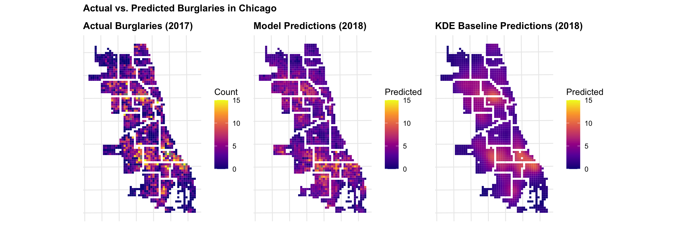
# Add predictions back to fishnet using existing model
fishnet_lights_morans <- fishnet_lights_morans %>%
  mutate(
    prediction_nb = predict(model_nb_burglary, fishnet_lights_morans, type = "response")
  )

cat("✓ Generated final model predictions\n")

✓ Generated final model predictions

cat("  - Mean predicted burglaries:", round(mean(fishnet_lights_morans$prediction_nb, na.rm = TRUE), 2), "\n")

  - Mean predicted burglaries: 3.81 

cat("  - Mean actual burglaries:", round(mean(fishnet_lights_morans$countBurglaries, na.rm = TRUE), 2), "\n")

  - Mean actual burglaries: 3.73 

Create KDE Baseline

Here, we create a simple baseline using Kernel Density Estimation (KDE). This is a simple baseline because it presents a null hypothesis that burglaries happen neaer where they happened before. If the more complicated model doesn’t outperform this, we need to work on it.

# Convert burglaries to ppp (point pattern) format for spatstat
burglaries_ppp <- as.ppp(
  st_coordinates(burglaries),
  W = as.owin(st_bbox(chicagoBoundary))
)

# Calculate KDE with 1000 ft bandwidth
kde_burglaries <- density.ppp(
  burglaries_ppp,
  sigma = 1000,  
  edge = TRUE
)

# Convert to terra raster
kde_raster <- rast(kde_burglaries)

# Extract KDE values to fishnet cells
fishnet_lights_morans <- fishnet_lights_morans %>%
  mutate(
    kde_value = terra::extract(
      kde_raster,
      vect(fishnet_lights_morans),
      fun = mean,
      na.rm = TRUE
    )[, 2]  # Extract just the values column
  )

# Normalize KDE to same scale as counts
kde_sum <- sum(fishnet_lights_morans$kde_value, na.rm = TRUE)
count_sum <- sum(fishnet_lights_morans$countBurglaries, na.rm = TRUE)

fishnet_lights_morans <- fishnet_lights_morans %>%
  mutate(
    prediction_kde = (kde_value / kde_sum) * count_sum
  )

Compare Model vs KDE Baseline

# Create three maps
p1 <- ggplot() +
  geom_sf(data = fishnet_lights_morans, aes(fill = countBurglaries), color = NA) +
  scale_fill_viridis_c(name = "Count", option = "plasma", limits = c(0, 15)) +
  labs(title = "Actual Burglaries (2017)") +
  theme_crime()

p2 <- ggplot() +
  geom_sf(data = fishnet_lights_morans, aes(fill = prediction_nb), color = NA) +
  scale_fill_viridis_c(name = "Predicted", option = "plasma", limits = c(0, 15)) +
  labs(title = "Model Predictions (2018)") +
  theme_crime()

p3 <- ggplot() +
  geom_sf(data = fishnet_lights_morans, aes(fill = prediction_kde), color = NA) +
  scale_fill_viridis_c(name = "Predicted", option = "plasma", limits = c(0, 15)) +
  labs(title = "KDE Baseline Predictions (2018)") +
  theme_crime()

p1 + p2 + p3 +
  plot_annotation(
    title = "Actual vs. Predicted Burglaries in Chicago",
  )

# Calculate performance metrics
comparison <- fishnet_lights_morans %>%
  st_drop_geometry() %>%
  filter(!is.na(prediction_nb), !is.na(prediction_kde)) %>%
  summarize(
    model_mae = mean(abs(countBurglaries - prediction_nb)),
    model_rmse = sqrt(mean((countBurglaries - prediction_nb)^2)),
    kde_mae = mean(abs(countBurglaries - prediction_kde)),
    kde_rmse = sqrt(mean((countBurglaries - prediction_kde)^2))
  )

comparison %>%
  pivot_longer(everything(), names_to = "metric", values_to = "value") %>%
  separate(metric, into = c("approach", "metric"), sep = "_") %>%
  pivot_wider(names_from = metric, values_from = value) %>%
  kable(
    digits = 2,
    caption = "Model Performance Comparison (2017)",
    col.names = c("Approach", "MAE", "RMSE")
  ) %>%
  kable_styling(bootstrap_options = c("striped", "hover", "condensed"))

Model Performance Comparison (2017)

Approach	MAE	RMSE
model	2.46	3.52
kde	2.14	3.01

Map Prediction Errors

# Calculate errors
fishnet_lights_morans <- fishnet_lights_morans %>%
  mutate(
    error_nb = countBurglaries - prediction_nb,
    error_kde = countBurglaries - prediction_kde,
    abs_error_nb = abs(error_nb),
    abs_error_kde = abs(error_kde)
  )

# Map errors for negative binomial model
p1 <- ggplot() +
  geom_sf(data = fishnet_lights_morans, aes(fill = error_nb), color = NA) +
  scale_fill_gradient2(
    name = "Error",
    low = "#2166ac", 
    mid = "white", 
    high = "#b2182b",
    midpoint = 0,
    limits = c(-10, 10)
  ) +
  labs(title = "Model Errors (Actual - Predicted)") +
  theme_crime()

p2 <- ggplot() +
  geom_sf(data = fishnet_lights_morans, aes(fill = abs_error_nb), color = NA) +
  scale_fill_viridis_c(name = "Abs. Error", option = "magma") +
  labs(title = "Absolute Model Errors") +
  theme_crime()

p1 + p2 +
  plot_annotation(
    title = "Where Does the Model Fail?",
    subtitle = "Red = Under-prediction (actual > predicted), Blue = Over-prediction"
  )

tibble(
  Metric = c("Mean Error", "Mean Absolute Error", "RMSE", "Max Over-prediction", "Max Under-prediction"),
  `Negative Binomial` = c(
    mean(fishnet_lights_morans$error_nb, na.rm = TRUE),
    mean(fishnet_lights_morans$abs_error_nb, na.rm = TRUE),
    sqrt(mean(fishnet_lights_morans$error_nb^2, na.rm = TRUE)),
    min(fishnet_lights_morans$error_nb, na.rm = TRUE),
    max(fishnet_lights_morans$error_nb, na.rm = TRUE)
  ),
  KDE = c(
    mean(fishnet_lights_morans$error_kde, na.rm = TRUE),
    mean(fishnet_lights_morans$abs_error_kde, na.rm = TRUE),
    sqrt(mean(fishnet_lights_morans$error_kde^2, na.rm = TRUE)),
    min(fishnet_lights_morans$error_kde, na.rm = TRUE),
    max(fishnet_lights_morans$error_kde, na.rm = TRUE)
  )
) %>%
  kable(
    digits = 2,
    caption = "Prediction Error Summary",
    format.args = list(big.mark = ",")
  ) %>%
  kable_styling(bootstrap_options = c("striped", "hover", "condensed"))

Prediction Error Summary

Metric	Negative Binomial	KDE
Mean Error	-0.08	0.00
Mean Absolute Error	2.46	2.14
RMSE	3.52	3.01
Max Over-prediction	-13.45	-7.76
Max Under-prediction	34.17	30.16