| DRINKING_D | Count | Proportion |
|---|---|---|
| 0 | 40879 | 0.943 |
| 1 | 2485 | 0.057 |
Homework 3: The Application of Logistic Regression to Examine the Predictors of Car Crashes Caused by Alcohol
1 Introduction
Car crashes involving alcohol-impaired driving are a major public safety issue in the United States, contributing to almost 30 deaths every day. Understanding the factors that make an alcohol-related crash more or less likely is critical towards deploying effective interventions. This report focuses on 43,364 crashes that occurred in Philadelphia’s residential block groups, where demographic and socioeconomic data is available, to study the association between alcohol-impaired driving crashes and certain predictors.
The predictors included in this study reflect both crash conditions and the characteristics of the surrounding neighborhood. Predictors such as speeding, aggressive driving, or a fatal or major-injury outcome were explored because of potential links to risky behavior that occurs with alcohol use, while age-related variables capture groups that are statistically over- or under-represented in drunk-driving crashes. Neighborhood indicators like median household income and educational attainment may also be associated with spatial patterns of alcohol-involved crashes. To examine these relationships, we use R to run a logistic regression model that predicts the probability that a given crash involved a drinking driver.
2 Methods
2.1 Logistic Regression Motivation and Foundation
The dependent variable in this report (DRINKING_D) is a binary indicator: it takes the value 1 (True) or 0 (False). This presents a major limitation for Ordinary Least Squares (OLS) regression. OLS assumes a continuous dependent variable and estimates coefficients that can take any value from \(-\infty\) to \(+\infty\), interpreting each coefficient as the expected change in the dependent variable for a one-unit increase in a predictor. When the outcome is binary, this interpretation breaks down. A predicted value of 0.65, for example, is not meaningful when the outcome can only be 0 or 1.
Because of these issues, logistic regression is more appropriate for modeling a binary outcome. Logistic regression works by transforming the probability of the event into a metric that can take any real value: the log-odds (also called the logit). To understand this transformation, it helps to introduce the concept of odds.
While probability is defined as \(\Pr(\text{event}) = \frac{\#\text{desirable outcomes}}{\#\text{possible outcomes}}\), the odds of an event are defined as \(\frac{\#\text{desirable outcomes}}{\#\text{undesirable outcomes}}\). In the context of this report, the odds of drink-driving are \(\frac{\#\text{with drink driving}}{\#\text{without drink driving}}\).
Logistic regression models the log of the odds, or the logit, as a linear function of the predictors. Because the log-odds range from \(-\infty\) to \(+\infty\), the model avoids the limitations of OLS. Exponentiating a logistic regression coefficient produces an odds ratio (OR), which describes how the odds of the outcome change for a one-unit increase in a predictor. An \(OR > 1\) indicates increased odds of the event, while an \(OR < 1\) indicates decreased odds.
To model the probability that a crash involved a drinking driver, we use a logistic regression model with DRINKING_D as the dependent variable and a set of binary and continuous predictors. The binary predictors indicate whether specific conditions applied to the crash: whether the crash resulted in a fatality or major injury (FATAL_OR_M), whether the vehicle was overturned (OVERTURNED), whether the driver was using a cell phone at the time of the crash (CELL_PHONE), whether the crash involved speeding (SPEEDING), whether aggressive driving was involved (AGGRESSIVE), whether at least one driver was 16 or 17 years old (DRIVER1617), or whether at least one driver was 65 or older (DRIVER65PLUS). In addition, the model includes continuous block-group-level predictors, specifically the percent of adults with at least a bachelor’s degree (PCTBACHMOR) and the median household income (MEDHHINC) for the location where the crash occurred. For this report, the logit model expresses the log-odds of a drinking-driver crash as a linear function of the predictors. The model is:
\[ \begin{aligned} \ln\left(\frac{p}{1 - p}\right) =\;& \beta_0 + \beta_1 \text{(FATAL OR M)} + \beta_2 \text{(OVERTURNED)} + \beta_3 \text{(CELL PHONE)} \\ &+ \beta_4 \text{(SPEEDING)} + \beta_5 \text{(AGGRESSIVE)} + \beta_6 \text{(DRIVER1617)} \\ &+ \beta_7 \text{(DRIVER65PLUS)} + \beta_8 \text{(PCTBACHMOR)} + \beta_9 \text{(MEDHHINC)}. \end{aligned} \]
Here, \(p\) is the probability that \(\text{DRINKING\_D} = 1\), meaning the crash involved a drinking driver. The term \(\ln\left(\frac{p}{1-p}\right)\) is the logit, or the natural log of the odds of a drinking-driver crash. Each \(\beta_k\) represents the change in the log-odds associated with a one-unit increase in the corresponding predictor, holding the others constant.
Binary predictors such as \(\text{FATAL\_OR\_M}\) or \(\text{SPEEDING}\) shift the log-odds by \(\beta_k\) when the indicator changes from 0 to 1. Continuous predictors such as \(\text{PCTBACHMOR}\) and \(\text{MEDHHINC}\) shift the log-odds proportionally to their values.
We can rewrite the model by solving for \(p = P(\text{DRINKING\_D} = 1)\) (note: to make the formula fit on the report, we used z to notate the \(\beta\) coefficients and predictors) :
\[ \begin{aligned} p &= \frac{1}{1 + e^{-z}} = \frac{e^z}{1 + e^z} \\[10pt] \text{where } z =\;& \beta_0 + \beta_1 \text{(FATAL OR M)} + \beta_2 \text{(OVERTURNED)} + \beta_3 \text{(CELL PHONE)} \\ &+ \beta_4 \text{(SPEEDING)} + \beta_5 \text{(AGGRESSIVE)} + \beta_6 \text{(DRIVER1617)} \\ &+ \beta_7 \text{(DRIVER65PLUS)} + \beta_8 \text{(PCTBACHMOR)} + \beta_9 \text{(MEDHHINC)} \end{aligned} \]
This expression uses the logistic function, which transforms any real-valued input into a valid probability between \(0\) and \(1\). The denominator, with the exponentiation, ensures that \(p\) is always bounded between \(0\) and \(1\), regardless of the values of the predictors or coefficients.
2.2 Hypothesis Testing Overview
In logistic regression, each predictor \(x_i\) is tested for the null hypothesis, \(H_0\), that the beta coefficient, \(\beta_i\), is 0 against the alternative hypothesis \(H_a\) that \(\beta_i\) is not 0: \[ H_0: \beta_i = 0 \] \[ H_a: \beta_i \neq 0 \] The z-value, also known as the Wald statistic in logistic regression, is the test statistic that we calculate under the null hypothesis. We calculate this statistic by dividing the estimated beta coefficient, \(\hat{\beta}_i\), by its standard error or \(\sigma_{\hat{\beta}_i}\):
\[ z = \frac{\hat{\beta}_i}{\sigma_{\hat{\beta}_i}} \]
Under the null hypothesis, the Wald statistic follows an approximately standard normal distribution, N(0,1). This property allows us to compute the two‑tailed p‑value as the probability of observing a statistic as extreme, or more extreme, than the calculated statistic if the null hypothesis were true. If the p-value is < 0.05, we can reject the null hypothesis in favor of the alternative hypothesis that \(\beta_i\) is not 0. Rather than interpreting the raw beta coefficients, statisticians prefer use the odds ratio, \(OR_i\), which can be calculated by exponentiating \(\hat{\beta}_i\):
\[ OR_i = e^{\hat{\beta}_i} \]
The odds ratio expresses the effect of a predictor on the dependent variable in multiplicative terms. Specifically, it represents how the odds of the event change for a one‑unit increase in the predictor, holding other variables constant. The null and alternative hypothesis can be adapted for the odds ratio, where the null hypothesis is the predictor has no effect on the odds (\(OR = 1\)) and the alternative hypothesis is that the predictor increases or decrease the odds of the event (\(OR \neq 1\)): \[ H_0: OR = 1 \] \[ H_a: OR \neq 1 \] Conceptually, the odds ratio is the ratio of the odds with the predictor present to the odds with the predictor absent. Thus, if the odds ratio equals 1, it indicates that the odds are the same: the predictor did not change the odds of the outcome. Alternatively, if the odds ratio is significantly above or below 1, the predictor increased or decreased the odds. The confidence intervals for the odds ratios can be calculated by exponentiating the coefficient confidence intervals. These intervals provide a range of plausible values for the true odds ratio, reflecting the uncertainty of the estimate. In the context of logistic regression, the presence of a 1 in the confidence interval indicates the predictor’s effect is not statistically significant while a confidence interval entirely above or below 1, indicates that the predictor increased or decreased the odds.
All coefficient estimates, z‑values, and p‑values were extracted in R from the fitted logistic regression model’s summary. Odds ratios and their confidence intervals were calculated by exponentiating the original coefficient estimates and confidence intervals, then merged with the extracted coefficients for interpretation.
2.3 Assessing Model Quality of Fit
In our analysis, goodness of the model’s fit was evaluated in various ways. In Ordinary Least Squares (OLS) regression, \(R^2\) is used to evaluate model fit as it is a statistic that returns the proportion of total variance in the dependent variable explained by the independent variable. Unlike in OLS regression, logistic regression doesn’t model a continuous outcome. In logistic regression the dependent variable, \(Y\) is binary, taking a value of 1 to indicate the occurrence of an event or 0 to indicate its absence. Therefore, since there is no longer a meaningful attribution of unexplained and explained variance in the dependent variable, \(R^2\) can no longer be interpreted as the percent of variance explained by the model. Similarly to linear regression, residuals, \(\varepsilon_i\), are calculated as the difference between the observed values of the dependent variable , \(y_i\), and the predicted values of the dependent variable, \(\hat{y}_i\): \[
\varepsilon_i = y_i - \hat{y}_i
\] In logistic regression, however, the predicted values, \(\hat{y}_i\), represent the probability that \(Y=1\) , while \(y_i\) represent the binary outcome (\(Y=1\) or \(Y=0\)). Thus, residuals represent the difference between the observed binary outcome and the model’s predicted probabilities. Theoretically a model of good fit predicts high probabilities of \(Y=1\) if \(y_i\) actually equals 1 and a low probability of \(Y=1\) if \(y_i\) is actually 0. In order to determine what is considered high probability and low probability, a cut-off value is imposed on the \(\hat{y}_i\) values. Cut-off values are then evaluated based on their specificity, sensitivity, and misclassification rates. Sensitivity, also called the true positive rate, is the proportion of actual positives that are correctly identified: \[
\text{Sensitivity} = \frac{\text{True Positives}}{\text{True Positives} + \text{False Negatives}}
\] In this analysis, the sensitivity rate is the proportion of observed \(y_i\) = 1 values correctly predicted as 1. Specificity, also called the true negative rate, is the proportion of actual negatives that are correctly identified as negatives: \[
\text{Specificity} = \frac{\text{True Negatives}}{\text{True Negatives} + \text{False Positives}}
\] The specificity rate in this analysis is the proportion of observed \(y_i\) = 0 values correctly predicted as 0. The misclassification rate is the proportion of incorrectly identified positive and negative \(y_i\) values based on the total number of predictions: \[
\text{Misclassification} = \frac{\text{False Negatives}+ \text{False Positives}}{\text{True Negatives} + \text{True Positives} + \text{False Positives} + \text{False Negatives}}
\] In R, we called upon fit.binary and set the fit parameter to various different values to simulate how various cut off values would impact the sensitivity, specification, and misclassification rate. In other words, we use multiple cut-off values to compare the trade-offs of each cut-off threshold. Ideally, the chosen threshold will achieve higher sensitivity and specificity while minimizing the misclassification rate.
Receiver Operating Characteristics (ROC) curves are another tool for evaluating cut-off values. The ROC curve plots sensitivity against the false positive rate (1 – specificity) across all possible cut-off values of \(\hat{y}_i\). The baseline for evaluating ROC curves called the “worthless” ROC is a 45 degree line where sensitivity and the false positive rate are equal across all cut-off values, meaning the predictions are no better than a random guess. Effective models produce ROC curves that lie above this diagonal baseline. ROC curves can be used to determine the cut-off value that balances the sensitivity and specificity rate, characteristics that indicate a good model. One common way to determine the optimal cut-off value is to use the Youden Index, which identifies the cut-off that maximizes the sum of sensitivity and specificity is maximized: \[ J = Sensitivity + Specificity - 1 \] This corresponds to the point on the ROC curve farthest above the diagonal line, or equivalently, the point closest to the top-left corner of the graph where sensitivity and specificity both equal 1. To identify the optimal cut‑off value, we implemented a function in R that is conceptually similar to the Youden Index as it attempts to find the point that minimizes the distance to this ideal point.
In addition to identifying an optimal cut‑off, we can also calculate Area Under Curve (AUC) for our ROC curve as a measure of the model’s overall predictive accuracy. The AUC quantifies the model’s ability to discriminate between positive and negative outcomes across all possible cut‑offs. An AUC of 1 (area of the entire graph) indicates perfect classification or discrimination while a value of 0.5 (area under the 45 degree line) indicates no better than random guessing. AUC can be interpreted as the probability that the model assigns a higher predicted probability to a randomly chosen positive case than to a randomly chosen negative case. Higher AUC values therefore reflect stronger overall discriminative ability across all possible cut‑off values, implying that at least one threshold exists where both sensitivity and specificity are relatively high. In this analysis, the AUC was computed in R using the performance function from the ROCR package. We relied on commonly established thresholds for evaluating model accuracy based on AUC values where 0.90–1.00 indicates excellent accuracy, 0.80–0.90 good, 0.70–0.80 fair, 0.60–0.70 poor, and 0.50–0.60 indicates the model failed.
Another measure used to evaluate logistic regression model fit is the Akaike Information Criterion (AIC). Although the absolute value of the AIC is not interpretable on its own, it provides a basis for comparing two or more models. Specifically, AIC combines the log‑likelihood of the predicted probabilities with a penalty for the number of estimated parameters. Lower AIC values indicate a more favorable balance between model complexity and goodness of fit.
2.4 Assumptions of Logistic Regression
Logistic regression models the relationship between a set of predictors and a binary dependent variable by expressing the log-odds of the outcome as a linear function of the predictors:
\[ \log\left(\frac{p}{1-p}\right) = \beta_0 + \beta_1X_1 + \cdots + \beta_kX_k. \]
The predicted probability of the outcome is obtained by applying the logistic transformation:
\[ p = \frac{e^{\eta}}{1 + e^{\eta}}, \qquad \eta = \beta_0 + \beta_1X_1 + \cdots + \beta_kX_k. \] Here, \(p\) represents the predicted probability of the event occurring, \(X_k\) are the predictor variables, and \(\beta_k\) are the corresponding regression coefficients. This formulation ensures that predicted probabilities remain between 0 and 1, while allowing the model to use a linear combination of predictors on the log-odds scale.
2.4.1 Logistic Regression Assumptions
Logistic regression shares several assumptions with Ordinary Least Squares (OLS) regression, while relaxing others. As in OLS, logistic regression assumes that observations are independent of one another. Independence ensures that the estimated coefficients and their standard errors are valid. The model also assumes that the predictors are not perfectly collinear. Severe multicollinearity inflates standard errors and reduces the reliability of coefficient estimates.
However, several OLS assumptions do not apply to logistic regression. Logistic regression does not assume homoscedasticity of residuals, because the variance of a binary dependent variable is a function of its mean. The model also does not require that residuals follow a normal distribution. In addition, the model does not assume a linear relationship between the predictors and the outcome on the original probability scale. Instead, it assumes linearity only in the log-odds, as shown in the equations above.
2.5 Exploratory Analyses Prior to Logistic Regression
Before fitting a logistic regression model, it is useful to assess the relationships among the predictors to ensure that they do not exhibit multicollinearity. To do this, Pearson correlation coefficients can be calculated between the continuous predictors and the dependent variable, as well as among the predictors themselves. Examining the magnitude of these correlations helps determine whether any predictors are highly correlated, which could inflate standard errors and affect coefficient stability in the logistic regression model.
2.5.1 Cross-tabulations for Binary Predictors
When both the dependent variable and a predictor are categorical, a cross-tabulation provides a simple way to examine the distribution of outcomes across different categories of the predictor. To formally test whether the distribution of the dependent variable varies across levels of a binary predictor, the appropriate statistical method is the Chi-Square (\(\chi^2\)) test of independence.
For the \(\chi^2\) test, the null hypothesis states that the two categorical variables are independent; that is, the proportion of positive and negative outcomes is the same for both levels of the predictor. The alternative hypothesis states that the variables are not independent, meaning that the distribution of the dependent variable differs across categories of the predictor. A large \(\chi^2\) statistic and a p-value below the conventional significance threshold (e.g., 0.05) provide evidence against the null hypothesis and suggest that an association exists between the two categorical variables.
2.5.2 Comparing Means of Continuous Predictors
For continuous predictors, it is often useful to compare their mean values across the two categories of the binary dependent variable. The appropriate statistical test for comparing the means of a continuous variable between two independent groups is the independent samples t-test.
For the t-test, the null hypothesis states that the mean value of the continuous predictor is the same across both groups of the dependent variable. The alternative hypothesis states that the means differ between the two groups. A large absolute value of the t-statistic and a p-value below the specified significance level (e.g., 0.05) provide evidence to reject the null hypothesis and conclude that there are significant differences in mean values between the groups.
3 Results
3.1 Exploratory Analysis
Before beginning the logistic regression, we must do some exploratory analysis of the data and check assumptions of the regression model. Below is a summary table of the dependent variable, displaying both the count and proportion of crashes that involved a drinking driver versus those that did not.
The distribution of the dependent variable shows that the vast majority of crashes did not involve a drinking driver: 40,879 crashes (94.3%). Only 2,485 crashes, or about 5.7%, involved a drinking driver.
It is also useful to examine the relationships between the dependent variable, DRINKING_D, and each of the binary predictors. Table 2 presents the cross-tabulations of DRINKING_D with each predictor, along with the proportion of crashes in each category. For each predictor, the table also includes the Chi-Square p-value to indicate whether the distribution of drinking-driver crashes differs significantly across its categories.
| Predictor | Num | Pct. | Num | Pct. | Total | Chi-square p-value |
|---|---|---|---|---|---|---|
| FATAL_OR_M | 1181 | 2.89% | 188 | 7.57% | 1369 | <0.001 |
| OVERTURNED | 612 | 1.50% | 110 | 4.43% | 722 | <0.001 |
| CELL_PHONE | 426 | 1.04% | 28 | 1.13% | 454 | 0.763 |
| SPEEDING | 1261 | 3.08% | 260 | 10.46% | 1521 | <0.001 |
| AGGRESSIVE | 18522 | 45.31% | 916 | 36.86% | 19438 | <0.001 |
| DRIVER1617 | 674 | 1.65% | 12 | 0.48% | 686 | <0.001 |
| DRIVER65PLUS | 4237 | 10.36% | 119 | 4.79% | 4356 | <0.001 |
The Chi-Square tests indicate whether there is a significant association between DRINKING_D and each binary predictor. For most predictors (FATAL_OR_M, OVERTURNED, SPEEDING, AGGRESSIVE, DRIVER1617, and DRIVER65PLUS) the p-values are less than 0.001, which is far below our significance threshold of 0.05. This allows us to reject the null hypothesis of independence for these variables, suggesting that the occurrence of a drinking-driver crash is significantly associated with these factors.
In contrast, the p-value for CELL_PHONE is 0.763, well above 0.05, indicating that we fail to reject the null hypothesis. There is no statistically significant association between drinking-driver crashes and whether the driver was using a cell phone at the time of the crash.
Overall, these results suggest that most of the binary predictors are significantly related to the likelihood of a crash involving a drinking driver, except for CELL_PHONE.
To further explore factors associated with drinking-driver crashes, we next examine the continuous predictors, PCTBACHMOR and MEDHHINC, comparing their means and standard deviation across crashes with and without alcohol involvement and conducting independent samples t-tests,
| Predictor | Mean | SD | Mean | SD | t-test p-value |
|---|---|---|---|---|---|
| PCTBACHMOR | 16.56986 | 18.21426 | 16.61173 | 18.72091 | 0.914 |
| MEDHHINC | 31483.05472 | 16930.10159 | 31998.75292 | 17810.49735 | 0.160 |
The summary statistics for the continuous predictors show that the mean percentage of individuals with a bachelor’s degree or higher (PCTBACHMOR) is very similar between crashes with no alcohol involvement (16.57%) and those with alcohol involvement (16.61%). The independent samples t-test yields a p-value of 0.914, which is far above our significance threshold of 0.05. This indicates that we fail to reject the null hypothesis, suggesting no significant difference in PCTBACHMOR between the two groups.
Similarly, the mean median household income (MEDHHINC) is slightly higher for alcohol-involved crashes ($31,998) compared to non-alcohol-involved crashes ($31,483), but the t-test p-value of 0.160 indicates that this difference is not statistically significant. Again, we fail to reject the null hypothesis, implying that MEDHHINC is not significantly associated with the likelihood of a crash involving a drinking driver.
Overall, the t-test results suggest that neither of the continuous predictors shows a significant association with DRINKING_D in this dataset.
3.2 Logistic Regression Assumption Checks
As previously mentioned, a key assumption of logistic regression is that there is no severe multicollinearity between predictors. We attempted to test whether our data violated this assumption by creating a pairwise Pearson coefficient matrix that included all our predictors.
Table 4 presents the Pearson correlation coefficients between all binary and continuous predictors. Pearson coefficients, \(r\), range from 1 to -1 and can be interpret as 1 indicating strong positive linear correlation, -1 indicating strong negative linear correlation, and 0 indicating no linear correlation. Because correlation coefficients are rarely perfectly negative or positive, the threshold considered to indicate moderate correlation is an absolute value of \(r\) (\(|r|\)) between 0.5 and 0.8 while \(|r|\) < 0.5 indicates weak correlation and \(|r|\) > 0.8 indicates strong correlation.
The coefficients that include binary variables are all uniformly small, near‑zero values. Because the Pearson correlation coefficient is designed to measure the strength of a linear relationship between continuous variables, it is not an ideal measure of association when applied to binary predictors. As a result, Pearson correlation is not as accurate for assessing relationships between binary predictors (or between binary and continuous predictors) and may misrepresent the true association. This means that in our analysis, while the Pearson coefficients are uniformly small, we must be cautious or explore an alternative method in interpreting them.
The correlation coefficient between the two continuous variables, PCTBACHMOR and MEDHHINC, is, as expected, the highest as \(r\)=0.478. Multicollinearity is considered to occur when two or more predictors are very strongly correlated (\(|r|\) > 0.9). The correlation between PCTBACHMOR and MEDHHINC is far below this threshold, suggesting no severe multicollinearity.
3.3 Logistic Regression Results
3.3.1 Logistic Regression with All Predictors
To identify the predictors associated with alcohol-related crashes, we estimated a logistic regression model that included all binary and continuous predictors. The estimated coefficients, p-values, and odds ratios are presented as shown below.
The logistic regression model includes all binary and continuous predictors. This model helps identify which factors are associated with crashes that involve alcohol. Table X presents the estimated coefficients, standard errors, p-values, odds ratios, and 95% confidence intervals for each predictor.
Several predictors are statistically significant. Crashes that resulted in a fatality or major injury show higher odds of involving alcohol, with an odds ratio of approximately 2.26. Crashes involving overturned vehicles are also more likely to involve alcohol, with an odds ratio of about 2.53. Speeding has the strongest association among all predictors, with an odds ratio of approximately 4.66, indicating substantially higher odds of alcohol involvement. Aggressive driving is negatively associated with alcohol involvement, with an odds ratio of 0.55. Both age-related indicators are significant: crashes involving 16–17-year-old drivers or drivers aged 65 or older have lower odds of involving alcohol, with odds ratios of 0.28 and 0.46, respectively.
Two predictors are not statistically significant in this model. Cell phone use does not show a meaningful association with alcohol involvement. The percentage of residents with at least a bachelor’s degree (PCTBACHMOR) is also non-significant, with an odds ratio close to 1. Median household income is statistically significant but has an odds ratio of 1.0000028, indicating a negligible substantive effect.
Overall, the model indicates that specific crash characteristics (fatality, overturning, and speeding) and driver demographics (teenage or senior drivers) are important predictors of alcohol involvement, while cell phone use and neighborhood-level sociodemographic variables contribute little additional explanatory power.
3.3.2 Sensitivity, Specificity, Misclassification
To evaluate model performance across different probability thresholds, we computed sensitivity, specificity, and the overall misclassification rate for each cut-off value. The results are summarized as shown below.
| Cutoff | TP | FN | TN | FP | Sensitivity | Specificity | Misclassification |
|---|---|---|---|---|---|---|---|
| 0.02 | 2444 | 41 | 2374 | 38505 | 0.984 | 0.058 | 0.889 |
| 0.03 | 2437 | 48 | 2613 | 38266 | 0.981 | 0.064 | 0.884 |
| 0.05 | 1826 | 659 | 19176 | 21703 | 0.735 | 0.469 | 0.516 |
| 0.07 | 550 | 1935 | 37356 | 3523 | 0.221 | 0.914 | 0.126 |
| 0.08 | 459 | 2026 | 38370 | 2509 | 0.185 | 0.939 | 0.105 |
| 0.09 | 418 | 2067 | 38670 | 2209 | 0.168 | 0.946 | 0.099 |
| 0.10 | 408 | 2077 | 38762 | 2117 | 0.164 | 0.948 | 0.097 |
| 0.15 | 259 | 2226 | 39743 | 1136 | 0.104 | 0.972 | 0.078 |
| 0.20 | 57 | 2428 | 40690 | 189 | 0.023 | 0.995 | 0.060 |
| 0.50 | 4 | 2481 | 40875 | 4 | 0.002 | 1.000 | 0.057 |
To further evaluate model performance, predicted probabilities were converted to binary classifications using a series of probability cut-offs ranging from 0.02 to 0.50. For each cut-off, a confusion matrix was generated, allowing the calculation of sensitivity, specificity, and the overall misclassification rate.
Sensitivity measures the proportion of alcohol-related crashes correctly identified by the model, while specificity measures the proportion of non–alcohol-related crashes correctly classified. The misclassification rate reflects the overall proportion of incorrect predictions. As expected, lower cut-off values result in higher sensitivity and lower specificity, while higher cut-offs reverse this pattern.
Across the tested cut-offs, the lowest misclassification rate occurred at a cut-off of 0.05, indicating that this threshold achieves the best balance between false positives and false negatives for this model. In contrast, extremely low or high cut-offs, such as 0.02 or 0.50, produce substantially higher misclassification rates and therefore perform less effectively as classification rules.
These results illustrate the importance of assessing multiple probability thresholds when evaluating logistic regression models. The optimal choice of cut-off depends on the tradeoff between sensitivity and specificity that is most appropriate for the application.
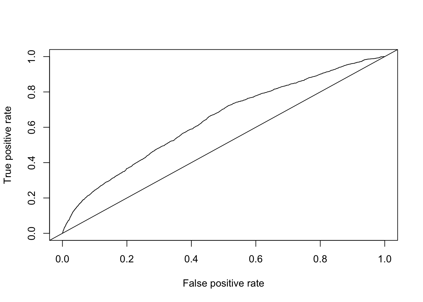
3.3.3 ROC curve & optimal cutoff
To evaluate the model’s ability to distinguish between alcohol-related and non–alcohol-related crashes, we generated a receiver operating characteristic (ROC) curve using the predicted probabilities from the full logistic regression model. The ROC curve shows the tradeoff between sensitivity and specificity across all possible probability thresholds, as shown below.
| Sensitivity | Specificity | Cutoff | |
|---|---|---|---|
| sensitivity | 0.661 | 0.545 | 0.0637 |
Using the distance-to-(0,1) criterion, we identified the probability cut-off that minimizes the distance to the upper-left corner of the ROC space. The optimal cut-off derived from this approach was approximately 0.06365. This value can be compared with the cut-off of 0.05 identified earlier as the point that yielded the lowest misclassification rate. The difference between these two thresholds reflects the fact that the ROC-based method jointly considers sensitivity and specificity, while the misclassification-based approach evaluates only the proportion of incorrect predictions. Because the two criteria optimize different aspects of model performance, they do not necessarily produce the same probability cut-off.
3.3.4 Area Under the Curve (AUC)
The area under the ROC curve (AUC) provides a summary measure of the model’s overall discriminative ability. The AUC for this model was 0.6399, as shown below, indicating modest ability to distinguish between alcohol-related and non–alcohol-related crashes. An AUC value of 0.5 suggests no discriminatory power, while values above 0.7 are typically considered acceptable. Thus, while the model performs better than random chance, its ability to accurately classify crashes based on alcohol involvement is limited.
| AUC |
|---|
| 0.63987 |
3.3.5 Reduced model
To assess whether the continuous predictors contributed meaningfully to model performance, we estimated a reduced logistic regression model that included only the binary predictors. The estimated coefficients and odds ratios for this reduced model are presented as shown below.
| Model | Df | AIC |
|---|---|---|
| full_logit | 10 | 18359.63 |
| binary_logit | 8 | 18360.47 |
The results of the binary-only model are largely consistent with the full model. Fatal or major injury crashes, overturned vehicles, and speeding remain strong positive predictors of alcohol involvement. Aggressive driving continues to show a negative association. Both age-related predictors—drivers aged 16–17 and drivers aged 65 or older—also remain significant and retain similar effect sizes. As in the full model, cell phone use is not a significant predictor of alcohol involvement.
Comparing the reduced model with the full model shows that removing the continuous predictors does not change the significance of any of the key crash-related or demographic variables. However, the full model has a slightly lower Akaike Information Criterion (AIC = 18359.63) than the reduced model (AIC = 18360.47). Because lower AIC values indicate better model fit, this comparison suggests that the full model provides a marginally better fit, even though the continuous predictors do not substantially alter the significance or magnitude of the main effects.
4 Discussion
In this analysis, we used logistic regression to predict the outcomes of our binary dependent variable, DRINKING_D, using several binary and continuous predictors: FATAL_OR_M, OVERTURNED, CELL_PHONE, SPEEDING, AGGRESSIVE, DRIVER1617, DRIVER65PLUS, PCTBACHMOR, and MEDHHINC. Prior to modeling, we performed exploratory analyses to evaluate the relationships between our predictors and the dependent variable as well as between the predictors themselves. Our exploratory analysis confirmed no severe multicollinearity between predictors and suggested that all predictors except for CELL_PHONE, PCTBACHMOR, and MEDHHINC had significant associations with DRINKING_D. We proceeded by initially creating and evaluating a logistic regression model that included all the original binary and continuous predictors before creating and comparing the performance of a reduced model with only binary predictors. We found that, based on AIC values, our full model was slightly better than our reduced model despite the inclusion of statistically insignificant predictors.
Some of the results were consistent with what we expected, while others were surprising. Fatal and overturned crashes, as well as speeding, were strong predictors of alcohol involvement. In contrast, aggressive driving and drivers aged 16–17 or 65+ were associated with lower odds of alcohol involvement. Cell phone use, education level, and median household income were not significant predictors. Overall, most behavioral and crash-severity effects were in the expected direction, though some demographic effects were less intuitive.
Although the dependent variable is relatively rare, the overall sample size is large, and the model includes predictors with sufficient variation across the dataset. In this context, standard logistic regression remains an appropriate choice because maximum likelihood estimation can still perform reasonably well when the total number of events is above a few hundred. The concern about rare-events bias mainly applies when the number of events is extremely small or when certain predictors have very few positive cases. In our analysis, the total number of alcohol-related crashes (2,485) far exceeds the minimum threshold commonly cited in the rare-events literature. Therefore, while methods such as penalized likelihood or Firth correction may provide slightly more conservative estimates for the rarest predictors, the standard logistic regression model is unlikely to be meaningfully distorted. The direction and significance of the main predictors also align with substantive expectations, suggesting that the logistic model is performing well for this dataset.
There are several limitations to this analysis. First, alcohol involvement is likely underreported in police crash data, especially in cases where a sobriety test was not administered. This underreporting may weaken the observed relationships between the predictors and the dependent variable. Second, the analysis is cross-sectional and does not account for exposure or driving frequency; we do not know whether certain groups simply drive more or less often, which could influence crash likelihood independently of alcohol use. Third, the neighborhood variables describe the census block group where the crash occurred rather than characteristics of the individuals involved. As a result, these variables may not accurately reflect the socioeconomic backgrounds of the drivers. Finally, some predictors contain very small counts among alcohol-related crashes, which may increase uncertainty in those coefficient estimates despite the relatively large sample size overall.